
Hide/Show the code
x <- rnorm(10) Computo Journal Format
To be used as a template for contributions to Computo
 ISSN 2824-7795


This document provides a template based on the quarto system for contributions to Computo. The github repository in itself provides a specific quarto extension useful for authors (and editors!).
This document provides a template based on the quarto system for contributions to Computo (Computo Team 2021). We show how Python (Perez et al. 2011) or R (R Core Team 2020) code can be included.
This section covers basic formatting guidelines. Quarto is a versatile formatting system for authoring HTML based on markdown, integrating \(\LaTeX\) and various code block interpreted either via Jupyter or Knitr (and thus deal with Python, R and many other langages). It relies on the Pandoc Markdown markup language.
We will only give some formatting elements. Authors can refer to the Quarto web page for a complete view of the formatting possibilities.
Quarto itself is a work-in-progress and a lot of bugs are constantly fixed or features added. As such, we recommend:
To render/compile a document, run quarto render. A document will be generated that includes both content and the output of any embedded code chunks within the document:
quarto render content.qmd # will render to htmlBold text or italic
But we can also do a numbered list
\(\LaTeX\) code is natively supported1, which makes it possible to use mathematical formulae:
will render
\[ f(x_1, \dots, x_n; \mu, \sigma^2) = \frac{1}{\sigma \sqrt{2\pi}} \exp{\left(- \frac{1}{2\sigma^2}\sum_{i=1}^n(x_i - \mu)^2\right)} \]
It is also possible to cross-reference an equation, see Equation 1:
\[ \begin{aligned} D_{x_N} & = \frac12 \left[\begin{array}{cc} x_L^\top & x_N^\top \end{array}\right] \, \left[\begin{array}{cc} L_L & B \\ B^\top & L_N \end{array}\right] \, \left[\begin{array}{c} x_L \\ x_N \end{array}\right] \\ & = \frac12 (x_L^\top L_L x_L + 2 x_N^\top B^\top x_L + x_N^\top L_N x_N), \end{aligned} \tag{1}\]
Quarto includes a nice support for theorems, with predefined prefix labels for theorems, lemmas, proposition, etc. see this page. Here is a simple example:
Theorem 1 (Strong law of large numbers) The sample average converges almost surely to the expected value:
\[\overline{X}_n\ \xrightarrow{\text{a.s.}}\ \mu \qquad\textrm{when}\ n \to \infty.\]
See Theorem 1.
Quarto uses either Jupyter or knitr to render code chunks. This can be triggered in the yaml header, e.g., for Jupyter (should be installed on your computer) use
---
title: "My Document"
author "Jane Doe"
jupyter: python3
---
For knitr (R + knitr must be installed on your computer)
---
title: "My Document"
author "Jane Doe"
---
You can use Jupyter for Python code and more. And R + KnitR for if you want to mix R with Python (via the package reticulate Ushey et al. (2020)).
R code (R Core Team 2020) chunks may be embedded as follows:
x <- rnorm(10)reticulate (Ushey et al. 2020) manages the Python side: declare the packages you need with py_require() and it provisions an isolated environment (via uv) the first time Python is actually used, no separate conda/virtualenv setup required.
import plotly.io as pio
import plotly.express as px

# Force a kaleido-based static renderer: the default auto-detected
# "notebook" renderer relies on IPython's rich display machinery, which
# isn't available in this R/knitr + reticulate execution context.
pio.renderers.default = "png"

df = px.data.tips()
fig = px.histogram(df, x="total_bill", y="tip", color="sex",
                   marginal="box", # or violin, rug
                   hover_data=df.columns)
figFor a demonstration of a line plot on a polar axis, see Figure 2
import numpy as np
import matplotlib.pyplot as plt

r = np.arange(0, 2, 0.01)
theta = 2 * np.pi * r
fig, ax = plt.subplots(
  subplot_kw = {'projection': 'polar'}
)
ax.plot(theta, r)
ax.set_rticks([0.5, 1, 1.5, 2])
ax.grid(True)
plt.show()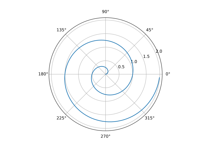
Plots can be generated as follows and referenced. See plot Figure 3:
library("ggplot2")
p <- ggplot(mpg, aes(displ, hwy)) +
  geom_point() +
  geom_smooth() + theme_bw()
p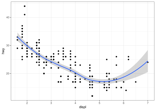
Plots combining semi-transparent layers with a viridis colour scale mapping missing values to a transparent colour (na.value = NA) render correctly in both formats, see Figure 4. Prior to v1.0.4, R’s Cairo-based svg() device (the previous HTML figure backend) emulated this kind of transparency through SVG filter chains that most browsers fail to render, showing a solid black rectangle instead of the plot; the HTML backend was switched to svglite, which supports transparency natively, to fix this.
library("ggplot2")
library("viridis")
set.seed(42)
df <- data.frame(x = rnorm(500), y = rnorm(500), v = rnorm(500))
df$v[sample(nrow(df), 50)] <- NA
ggplot(df, aes(x, y)) +
  geom_ribbon(aes(ymin = -2, ymax = 2), fill = "red", alpha = 0.2) +
  geom_point(aes(color = v), size = 2, shape = 15) +
  scale_color_viridis(na.value = NA) +
  theme_bw()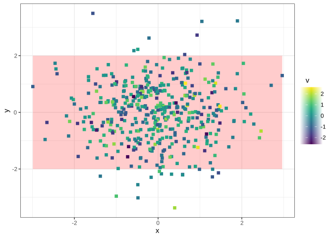
Interactive plots may also be produced in the HTML output of the document2:
library("plotly")
ggplotly(p)It is also possible to create figures from static images:

Tables (with label: @tbl-mylabel renders Table 1) can be generated with markdown as follows
| Tables   |      Are      |  Cool |
|----------|:-------------:|------:|
| col 1 is |  left-aligned | $1600 |
| col 2 is |    centered   |   $12 |
| col 3 is | right-aligned |    $1 |
: my table caption {#tbl-mylabel}| Tables | Are | Cool |
|---|---|---|
| col 1 is | left-aligned | $1600 |
| col 2 is | centered | $12 |
| col 3 is | right-aligned | $1 |
We also integrate the list tables filter from Pandoc, so that you may alternatively use this format , easier to write and maintain:
:::list-table
   * - row 1, column 1
     - row 1, column 2
     - row 1, column 3

   * - row 2, column 1
     -
     - row 2, column 3

   * - row 3, column 1
     - row 3, column 2
:::| row 1, column 1 | row 1, column 2 | row 1, column 3 |
|---|---|---|
| row 2, column 1 | row 2, column 3 | |
| row 3, column 1 | row 3, column 2 |
Table can also be generated by some code, for instance with knitr here:
knitr::kable(summary(cars), caption = "Table caption.")| speed | dist | |
|---|---|---|
| Min. : 4.0 | Min. : 2.00 | |
| 1st Qu.:12.0 | 1st Qu.: 26.00 | |
| Median :15.0 | Median : 36.00 | |
| Mean :15.4 | Mean : 42.98 | |
| 3rd Qu.:19.0 | 3rd Qu.: 56.00 | |
| Max. :25.0 | Max. :120.00 |
A solution to typeset pseudocode just like you would do with \(\LaTeX\), yet with HTML output is to rely on the JavaScript pseudocode.js. Your pseudocode is written inside a Code Block with the pseudocode class. Do not forget the class tag, that will trigger the rendering process of your pseudo-code. The result is as follows3:
```pseudocode
#| label: algo-quicksort
#| html-indent-size: "1.2em"
#| html-comment-delimiter: "//"
#| html-line-number: true
#| html-line-number-punc: ":"
#| html-no-end: false
#| pdf-placement: "htb!"
#| pdf-line-number: true

\begin{algorithm}
\caption{Quicksort}
\begin{algorithmic}
\Procedure{Quicksort}{$A, p, r$}
  \If{$p < r$}
    \State $q = $ \Call{Partition}{$A, p, r$}
    \State \Call{Quicksort}{$A, p, q - 1$}
    \State \Call{Quicksort}{$A, q + 1, r$}
  \EndIf
\EndProcedure
\Procedure{Partition}{$A, p, r$}
  \State $x = A[r]$
  \State $i = p - 1$
  \For{$j = p, \dots, r - 1$}
    \If{$A[j] < x$}
      \State $i = i + 1$
      \State exchange
      $A[i]$ with     $A[j]$
    \EndIf
    \State exchange $A[i]$ with $A[r]$
  \EndFor
\EndProcedure
\end{algorithmic}
\end{algorithm}
```Algorithm 1 is extracted from Chapter 7, Introduction to Algorithms (3rd edition).
In addition of quarto supported diagrams, we also support tikz diagrams. The following example4 is rendered as follows.
:::{#fig-tikz}

``` tikz
%%| filename: ../figure-tikz/fig-tikz
\begin{tikzpicture}[node distance=2cm, auto, thick, scale=2, every node/.style={transform shape}]
\node (P) {$P$};
\node (B) [right of=P] {$B$};
\node (A) [below of=P] {$A$};
\node (C) [below of=B] {$C$};
\node (P1) [node distance=1.4cm, left of=P, above of=P] {$\hat{P}$};
\draw[->] (P) to node {$f$} (B);
\draw[->] (P) to node [swap] {$g$} (A);
\draw[->] (A) to node [swap] {$f$} (C);
\draw[->] (B) to node {$g$} (C);
\draw[->, bend right] (P1) to node [swap] {$\hat{g}$} (A);
\draw[->, bend left] (P1) to node {$\hat{f}$} (B);
\draw[->, dashed] (P1) to node {$k$} (P);
\end{tikzpicture}
```

A simple example of a commutative diagram with $\texttt{tikz}$.

:::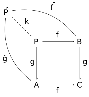
You may refer to it as Figure 7.
References are displayed as footnotes using BibTeX, e.g. [@computo] will be displayed as (Computo Team 2021), where computo is the bibtex key for this specific entry. The bibliographic information is automatically retrieved from the .bib file specified in the header of this document (here:references.bib).
As already (partially) seen, Quarto includes a mecanism similar to the bibliographic references for sections, equations, theorems, figures, lists, etc. Have a look at this page.
To go into more involved details, you can also simply check the source code of this document (button at the top), or have a look at the source of our t-sne remake example.
The pdf output is just a screenshot of the interactive plot from the html output↩︎
For proper pdf rendering, use Camel cased names for all algorithmic keywords, not upper case ones, like the examples in pseudocode.js’s documentation, which are not compatible with LaTeX.↩︎
This is the new syntax for cross-references since quarto 1.4, see Crossreferenceable elements↩︎
@article{computo_team2023,
  author = {Computo Team, The and friend, a},
  title = {Computo {Journal} {Format}},
  journal = {Computo},
  date = {2023-01-02},
  doi = {10.5072/computo.0000},
  issn = {2824-7795},
  langid = {en},
  abstract = {This document provides a template based on the quarto
    system for contributions to Computo. The github repository in itself
    provides a specific quarto extension useful for authors (and
    editors!).}
}