# Introduction
Litter pollution concerns every part of the globe. Each year, almost ten
thousand million tons of plastic waste is generated, among which 80\% ends up
in landfills or in nature (@geyer2017), notably threatening all of the
world’s oceans, seas and aquatic environments (@welden2020, @gamage2020).
Plastic pollution is known to already impact more than 3763 marine species
worldwide (see [this](https://litterbase.awi.de/) detailed analysis) with risk
of proliferation through the whole food chain. This accumulation of waste is
the endpoint of the largely misunderstood path of trash, mainly coming from
land-based sources (@rochman2016), yet rivers have been identified as a
major pathway for the introduction of waste into marine environments
(@jambeck2015). Therefore, field data on rivers and monitoring are
strongly needed to assess the impact of measures that can be taken. The
analysis of such field data over time is pivotal to understand the efficiency
of the actions implemented such as choosing zero-waste alternatives to
plastic, designing new products to be long-lasting or reusable, introducing
policies to reduce over-packing.
Different methods have already been tested to monitor waste in rivers: litter
collection and sorting on riverbanks (@Bruge2018), visual counting of
drifting litter from bridges (@gonzales2021), floating booms
(@gasperi2014), and nets (@moritt2014). All are helpful to understand
the origin and typology of litter pollution yet hardly compatible with long
term monitoring at country scales. Monitoring tools need to be reliable, easy
to set up on various types of rivers, and should give an overview of plastic
pollution during peak discharge to help locate hotspots and provide trends.
Newer studies suggest that plastic debris transport could be better understood
by counting litter trapped on river banks, providing a good indication of the
local macrolitter pollution especially after increased river discharge
(@VanEmmerik2019, @VanEmmerik2020). Based on these findings, we propose a
new method for litter monitoring which relies on videos of river banks
directly captured from moving boats.
In this case, object detection with deep neural networks (DNNs) may be used,
but new challenges arise. First, available data is still scarce. When
considering entire portions of river banks from many different locations, the
variety of scenes, viewing angles and/or light conditions is not well covered
by existing plastic litter datasets like (@Proenca2020), where litter is
usually captured from relatively close distances and many times in urban or
domestic backgrounds. Therefore, achieving robust object detection across
multiple conditions is still delicate.
Second, counting from videos is a different task than counting from
independent images, because individual objects will typically appear in
several consecutive frames, yet they must only be counted once. This last
problem of association has been extensively studied for the multi-object
tracking (MOT) task, which aims at recovering individual trajectories for
objects in videos. When successful MOT is achieved, counting objects in videos
is equivalent to counting the number of estimated trajectories. Deep learning
has been increasingly used to improve MOT solutions (@Ciaparrone2020b).
However, newer state-of-the-art techniques require increasingly heavy and
costly supervision, typically all object positions provided at every frame. In
addition, many successful techniques (@bergmann2019) can hardly be used
in scenarios with abrupt and nonlinear camera motion. Finally, while research
is still active to rigorously evaluate performance at multi-object *tracking*
(@luiten2020), most but not all aspects of the latter may affect global
video counts, which calls for a separate evaluation protocol dedicated to
multi-object *counting*.
Our contribution can be summarized as follows.
1. We provide a novel open-source image dataset of macro litter, which includes various objects seen from different rivers and different contexts.
This dataset was produced with a new open-sourced platform for data gathering and annotation developed in conjunction with Surfrider Foundation Europe, continuously growing with more data.
2. We propose a new algorithm specifically tailored to count in videos with fast camera movements.
In a nutshell, DNN-based object detection is paired with a robust state space movement model which uses optical flow to perform Bayesian filtering, while confidence regions built on posterior predictive distributions are used for data association.
This framework does not require video annotations at training time: the multi-object tracking module does not require supervision, only the DNN-based object detection does require annotated images.
It also fully leverages optical flow estimates and the uncertainty provided by Bayesian predictions to recover object identities even when detection recall is low.
Contrary to existing MOT solutions, this method ensures that tracks are stable enough to avoid repeated counting of the same object.
3. We provide a set of video sequences where litter counts are known and depicted in real conditions.
For these videos only, litter positions are manually annotated at every frame in order to carefully analyze performance.
This allows us to build new informative count metrics.
We compare the count performance of our method against other MOT-based alternatives.
A first visual illustration of the second claim is presented via the following code chunks: on three selected frames, we present a typical scenario where our strategy can avoid overcounting the same object (we depict internal workings of our solution against the end result of the competitors).
```{python}
#| label: fig-demo
#| fig-cap: "*Our method*: one object (red dot) is correctly detected at every frame and given a consistent identity throughout the sequence with low location uncertainty (red ellipse). Next to it, a false positive detection is generated at the first frame (brown dot) but immediatly lost in the following frames: the associated uncertainty grows fast (brown ellipse). In our solution, this type of track will not be counted. A third correctly detected object (pink) appears in the third frame and begins a new track."
import matplotlib
import matplotlib.pyplot as plt
import os
import pandas as pd
from surfnet.prepare_data import download_data
from surfnet.track import default_args as args

import pickle
import numpy as np

params = {'legend.fontsize': 'xx-large',
         'axes.labelsize': 'xx-large',
         'axes.titlesize':'xx-large',
         'xtick.labelsize':'xx-large',
         'ytick.labelsize':'xx-large'}
plt.rcParams.update(params)

# download frames and detections from a given deep detector model
download_data()

# prepare arguments
args.external_detections = True
args.data_dir = 'data/external_detections/part_1_segment_0'
args.output_dir = 'surfnet/results'
args.noise_covariances_path = 'surfnet/data/tracking_parameters'
args.confidence_threshold = 0.5
args.algorithm = 'EKF'
args.ratio = 4
args.display = 0


from surfnet.tracking.utils import resize_external_detections, write_tracking_results_to_file
from surfnet.tools.video_readers import FramesWithInfo
from surfnet.tracking.trackers import get_tracker
from surfnet.track import track_video

# Initialize variances
transition_variance = np.load(os.path.join(args.noise_covariances_path, 'transition_variance.npy'))
observation_variance = np.load(os.path.join(args.noise_covariances_path, 'observation_variance.npy'))

# Get tracker algorithm
engine = get_tracker(args.algorithm)

# Open data: detections and frames
with open(os.path.join(args.data_dir, 'saved_detections.pickle'),'rb') as f:
    detections = pickle.load(f)
with open(os.path.join(args.data_dir, 'saved_frames.pickle'),'rb') as f:
    frames = pickle.load(f)

# Create frame reader and resize detections
reader = FramesWithInfo(frames)
detections = resize_external_detections(detections, args.ratio)

# Start tracking, storing intermediate tracklets
results, frame_to_trackers = track_video(reader, detections, args, engine,
                                         transition_variance, observation_variance, return_trackers=True)

# Write final results
write_tracking_results_to_file(results, ratio_x=args.ratio, ratio_y=args.ratio, output_filename=args.output_dir)

from surfnet.track import build_image_trackers
# Choose a few indices to display (same for our algorithm and SORT)
idxs = [108, 112, 117]

considered_frames = [frames[i] for i in idxs]
considered_trackers = [frame_to_trackers[i] for i in idxs]
fig = build_image_trackers(considered_frames, considered_trackers, args, reader)
```
```{python}
## Tracker with SORT
from collections import defaultdict
import cv2
from sort.sort import track as sort_tracker

print('Tracking with SORT...')
print('--- Begin SORT internal logs')
sort_tracker(detections_dir='data/external_detections', output_dir='sort/results')
print('--- End')

def read_sort_output(filename):
    """ Reads the output .txt of Sort (or other tracking algorithm)
    """
    dict_frames = defaultdict(list)
    with open(filename) as f:
        for line in f:
            items = line[:-1].split(",")
            frame = int(items[0])
            objnum = int(items[1])
            x = float(items[2])
            y = float(items[3])
            dict_frames[int(items[0])].append((objnum, x, y))
    return  dict_frames


def build_image(frames, trackers, image_shape=(135,240), downsampling=2*4):
    """ Builds a full image with consecutive frames and their displayed trackers
    frames: a list of K np.array
    trackers: a list of K trackers. Each tracker is a per frame list of tracked objects
    """
    K = len(frames)
    assert len(trackers) == K
    font = cv2.FONT_HERSHEY_COMPLEX
    output_img=np.zeros((image_shape[0], image_shape[1]*K, 3), dtype=np.uint8)
    object_ids = []
    for tracker in trackers:
        for detection in tracker:
            object_ids.append(detection[0])
    min_object_id = min(object_ids)
    for i in range(K):
        frame = cv2.cvtColor(cv2.resize(frames[i], image_shape[::-1]), cv2.COLOR_BGR2RGB)
        for detection in trackers[i]:
            cv2.putText(frame, f'{detection[0]-min_object_id +1}', (int(detection[1]/downsampling)+10, int(detection[2]/downsampling)+10), font, 0.5, (255, 0, 0), 1, cv2.LINE_AA)

        output_img[:,i*image_shape[1]:(i+1)*image_shape[1],:] = frame
    return output_img
```
```{python}
#| label: fig-demo-sort
#| fig-cap: "*SORT*: the resulting count is also 2, but both counts arise from tracks generated by the same object, the latter not re-associated at all in the second frame. Additionally, the third object is discarded (in post-processing) by their strategy."
# open sort output
tracker_file = "sort/results/part_1_segment_0.txt"
frame_to_track = read_sort_output(tracker_file)

condisered_frames = [frames[idx] for idx in idxs]
considered_tracks = [frame_to_track[i] for i in idxs]
out_img = build_image(condisered_frames, considered_tracks)
plt.figure(figsize=(15,6))
plt.imshow(out_img)
plt.axis("off");
plt.show()
```
# Related works
## AI-automated counting
Counting from images has been an ongoing challenge in computer vision. Most
works can be divided into (i) detection-based methods where objects are
individually located for counting, (ii) density-based methods where counts are
obtained by summing a predicted density map, and (iii) regression-based
methods where counts are directly regressed from input images
(@Chattopadhyay). While some of these works tackled the problem of
counting in wild scenes (@Arteta2016), most are focused on pedestrian and
crowd counting. Though several works (@wu2020fast, @Xiong2017, @Miao2019)
showed the relevance of leveraging sequential inter-frame information to
achieve better counts at every frame, none of these methods actually attempt
to produce global video counts.
## Computer vision for macro litter monitoring
Automatic macro litter monitoring in rivers is still a relatively nascent
initiative, yet there have already been several attempts at using DNN-based
object recognition tools to count plastic trash. Recently, (@Proenca2020)
used a combination of two Convolutional Neural Networks (CNNs) to detect and
quantify plastic litter using geospatial images from Cambodia. In
(@Wolf2020), reliable estimates of plastic density were obtained using
Faster R-CNN (@ren2016faster) on images extracted from bridge-mounted
cameras. For underwater waste monitoring, (@vanlieshout2020automated)
assembled a dataset with bounding box annotations, and showed promising
performance with several object detectors. They later turned to generative
models to obtain more synthetic data from a small dataset @(Hong2020).
While proving the practicality of deep learning for automatic waste detection
in various contexts, these works only provide counts for separate images of
photographed litter. To the best of our knowledge, no solution has been
proposed to count litter directly in videos.
## Multi-object tracking
Multi-object tracking usually involves object detection, data association and
track management, with a very large number of methods already existing before
DNNs (@luo2021). MOT approaches now mostly differ in the level of
supervision they require for each step: until recently, most successful
methods (like @Bewley2016 have been detection-based, i.e. involving
only a DNN-based object detector trained at the image level and coupled with
an unsupervised data association step. In specific fields such as pedestrian
tracking or autonomous driving, vast datasets now provide precise object
localisation and identities throughout entire videos (@Caesar2020)
@Dendorfer2020). Current state-of-the-art methods leverage this supervision via
deep visual feature extraction (@Wojke2018, @Zhanga) or even self-attention
(@Chu2021) and graph neural networks (@Wang2021). For these
applications, motion prediction may be required, yet well-trained appearance
models are usually enough to deal with detection failures under simple motion,
therefore the linear constant-velocity assumption often prevails
(@Ciaparrone2020b).
In the case of macrolitter monitoring, however, available image datasets are
still orders of magnitude smaller, and annotated video datasets do not exist
at all. Even more so, real shooting conditions induce chaotic movements on the
boat-embedded cameras. A close work of ours is that of (@Fulton2018), who
paired Kalman filtering with optical flow to yield fruit count estimates on
entire video sequences captured by moving robots. However, their video footage
is captured at night with consistent lighting conditions, backgrounds are
largely similar across sequences, and camera movements are less challenging.
In our application context, we find that using MOT for the task of counting
objects requires a new movement model, to take into account missing detections
and large camera movements.
# Datasets for training and evaluation
Our main dataset of annotated images is used to train the object detector.
Then, only for evaluation purposes, we provide videos with annotated object
positions and known global counts. Our motivation is to avoid relying on
training data that requires this resource-consuming process.
## Images
### Data collection
With help from volunteers, we compile photographs of litter stranded on river
banks after increased river discharge, shot directly from kayaks navigating at
varying distances from the shore. Images span multiple rivers with various
levels of water current, on different seasons, mostly in southwestern France.
The resulting pictures depict trash items under the same conditions as the
video footage we wish to count on, while spanning a wide variety of
backgrounds, light conditions, viewing angles and picture quality.
### Bounding box annotation
For object detection applications, the images are annotated using a custom
online platform where each object is located using a bounding box. In this
work, we focus only on litter counting without classification, however the
annotated objects are already classified into specific categories which are
described in @fig-trash-categories-image.
A few samples are depicted below:
```{python}
from PIL import Image, ExifTags
from pycocotools.coco import COCO


def draw_bbox(image, anns, ratio):
    """
    Display the specified annotations.
    """
    for ann in anns:
        [bbox_x, bbox_y, bbox_w, bbox_h] = (ratio*np.array(ann['bbox'])).astype(int)
        cv2.rectangle(image, (bbox_x,bbox_y),(bbox_x+bbox_w,bbox_y+bbox_h), color=(0,0,255),thickness=3)

    return image

dir = 'surfnet/data/images'

ann_dir = os.path.join(dir,'annotations')
data_dir = os.path.join(dir,'images')
ann_file = os.path.join(ann_dir, 'subset_of_annotations.json')
coco = COCO(ann_file)

imgIds = np.array(coco.getImgIds())
print('{} images loaded'.format(len(imgIds)))

for imgId in imgIds:
    plt.figure()
    image = coco.loadImgs(ids=[imgId])[0]
    try:
        image = Image.open(os.path.join(data_dir,image['file_name']))
        # Rotation of the picture in the Exif tags
        for orientation in ExifTags.TAGS.keys():
            if ExifTags.TAGS[orientation]=='Orientation':
                break

        exif = image._getexif()
        if exif is not None:
            if exif[orientation] == 3:
                image=image.rotate(180, expand=True)
            elif exif[orientation] == 6:
                image=image.rotate(270, expand=True)
            elif exif[orientation] == 8:
                image=image.rotate(90, expand=True)

    except (AttributeError, KeyError, IndexError):
        # cases: image don't have getexif
        pass
    image = cv2.cvtColor(np.array(image.convert('RGB')),  cv2.COLOR_RGB2BGR)
    annIds = coco.getAnnIds(imgIds=[imgId])
    anns = coco.loadAnns(ids=annIds)
    h,w = image.shape[:-1]
    target_h = 1080
    ratio = target_h/h
    target_w = int(ratio*w)
    image = cv2.resize(image,(target_w,target_h))
    image = draw_bbox(image,anns,ratio)
    image = cv2.cvtColor(image,cv2.COLOR_BGR2RGB)
    plt.imshow(image)
    plt.axis('off')
```
## Video sequences
### Data collection
For evaluation, an on-field study was conducted with 20 volunteers to manually
count litter along three different riverbank sections in April 2021, on the
Gave d'Oloron near Auterrive (Pyrénées-Atlantiques, France), using kayaks. The
river sections, each 500 meters long, were precisely defined for their
differences in background, vegetation, river current, light conditions and
accessibility (see @sec-video-dataset-appendix for aerial views of
the shooting site and details on the river sections). In total, the three
videos amount to 20 minutes of footage at 24 frames per second (fps) and a
resolution of 1920x1080 pixels.
### Track annotation
On video footage, we manually recovered all visible object trajectories on
each river section using an online video annotation tool (more details
in @sec-video-dataset-appendix for the precise methodology). From that, we
obtained a collection of distinct object tracks spanning the entire footage.
# Optical flow-based counting via Bayesian filtering and confidence regions
Our counting method is divided into several interacting blocks. First, a
detector outputs a set of predicted positions for objects in the current
frame. The second block is a tracking module designing consistent trajectories
of potential objects within the video. At each frame, a third block links the
successive detections together using confidence regions provided by the
tracking module, proposing distinct tracks for each object. A final
postprocessing step only keeps the best tracks which are enumerated to yield
the final count.
## Detector
### Center-based anchor-free detection
In most benchmarks, the prediction quality of object attributes like bounding
boxes is often used to improve tracking. For counting, however, point
detection is theoretically enough and advantageous in many ways. First, to
build large datasets, a method which only requires the lightest annotation
format may benefit from more data due to annotation ease. Second, contrary to
previous popular methods (@ren2016faster) involving intricate mechanisms
for bounding box prediction, center-based and anchor-free detectors
(@Zhou2019, @Law) only use additional regression heads which can simply be
removed for point detection. Adding to all this, (@Zhanga) highlight
conceptual and experimental reasons to favor anchor-free detection in
tracking-related tasks.
For these reasons, we use a stripped version of CenterNet (@Zhou2019)
where offset and bounding box regression heads are discarded to output bare
estimates of center positions on a coarse grid. An encoder-decoder network
takes an input image $I \in [0,1]^{w \times h \times 3}$ (an RGB image of
width $w$ and height $h$), and produces a heatmap $\hat{Y} \in [0,1]^{\lfloor
w/p\rfloor \times \lfloor h/p\rfloor}$ such that $\hat{Y}_{xy}$ is the
probability that $(x,y)$ is the center of an object ($p$ being a stride
coefficient). At inference, peak detection and thresholding are applied to
$\hat{Y}$, yielding the set of detections. The bulk of this detector relies on
the DLA34 architecture (@fisher2017). In a video, for each frame $I_n \in
[0,1]^{w \times h \times 3}$ (where $n$ indexes the frame number), the
detector outputs a set $\mathcal{D}_n = \{z_n^i\}_{1 \leq i \leq D_n}$ where
each $z_n^i = (x_n^i,y_n^i)$ specifies the coordinates of one of the $D_n$
detected objects.
## Training {#sec-detector_training}
Training the detector is done similarly as in @Proenca2020.
For every image, the corresponding set $\mathcal{B} =
\{(c^w_i,c^h_i,w_i,h_i)\}_{1 \leq i\leq B}$ of $B$ annotated bounding boxes --
*i.e.* a center $(c^w_i,c^h_i)$, a width $w_i$ and a height $h_i$-- is
rendered into a ground truth heatmap $Y \in [0,1]^{{\lfloor w/p\rfloor \times
\lfloor h/p\rfloor}}$ by applying kernels at the bounding box centers and
taking element-wise maximum. For all $1 \leq x \leq w/p$, $1 \leq y \leq h/p$,
the ground truth at $(x,y)$ is
$$
Y_{xy} = \max\limits_{1\leq i\leq B}\left(\exp\left\{-\frac{(x-c_i^w)^2+(y-c_i^h)^2}{2\sigma^2_i}\right\}\right),
$$
where $\sigma_i$ is a parameter depending on the size of the object.
Training the detector is done by minimizing a penalty-reduced weighted focal loss
$$
\mathcal{L}(\hat{Y},Y) = -\sum_{x,y} \gamma_{xy}^\beta\left(1-\hat{p}_{xy}\right)^\alpha \log{\left(\hat{p}_{xy}\right)},
$$
where $\alpha$, $\beta$ are hyperparameters and
$$
(\hat{p}_{xy},\gamma_{xy}) = \left\{
\begin{array}{ll}
(\hat{Y}_{xy},1) & \mbox{if } Y_{xy} = 1, \\
(1 - \hat{Y}_{xy},1 - Y_{xy}) & \mbox{otherwise.}
\end{array}
\right.
$$
## Bayesian tracking with optical flow {#sec-bayesian_tracking}
### Optical flow
Between two timesteps $n-1$ and $n$, the optical flow $\Delta_n$ is a mapping
satisfying the following consistency constraint (@paragios2006):
$$
\widetilde{I}_n[u] = \widetilde{I}_{n-1}[u+\Delta_n(u)],
$$
where, in our case, $\widetilde{I}_n$ denotes the frame $n$ downsampled to
dimensions $\lfloor w/p\rfloor \times \lfloor h/p\rfloor$ and $u = (x,y)$ is a
coordinate on that grid. To estimate $\Delta_n$, we choose a simple
unsupervised Gunner-Farneback algorithm which does not require further
annotations, see @farneback2003two for details.
### State space model {#sec-state_space_model}
Using optical flow as a building block, we posit a state space model where
estimates of $\Delta_n$ are used as a time and state-dependent offset for the
state transition.
Let $(X_k)_{k \geq 1}$ and $(Z_k)_{k \geq 1}$ be the true (but hidden) and
observed (detected) positions of a target object in $\mathbb{R}^2$, respectively.
Considering the optical flow value associated with $X_{k-1}$ on the discrete
grid of dimensions $\lfloor w/p\rfloor \times \lfloor h/p\rfloor$, write
$$
X_k = X_{k-1} + \Delta_k(\lfloor X_{k-1} \rfloor) + \eta_k
$$ {#eq-state-transition}
and
$$
Z_k = X_k + \varepsilon_k,
$$
where $(\eta_k)_{k\geq 1}$ are i.i.d. centered Gaussian random variables with
covariance matrix $Q$ independent of $(\varepsilon_k)_{k\geq 1}$ i.i.d.
centered Gaussian random variables with covariance matrix $R$.
In the following, $Q$ and $R$ are assumed to be diagonal, and are
hyperparameters set to values given in @sec-covariance_matrices.
### Approximations of the filtering distributions
Denoting $u_{1:k} = (u_1,\ldots,u_k)$ for any $k$ and sequence $(u_i)_{i \geq
0}$, Bayesian filtering aims at computing the conditional distribution of
$X_k$ given $Z_{1:k}$, referred to as the filtering distribution. In the case
of linear and Gaussian state space models, this distribution is known to be
Gaussian, and Kalman filtering allows to update exactly the posterior mean
$\mu_k = \mathbb{E}[X_k|Z_{1:k}]$ and posterior variance matrix $\Sigma_k =
\mathbb{V}[X_k|Z_{1:k}]$. This algorithm and its extensions are prevalent and used
extensively in time-series and sequential-data analysis. As the transition
model proposed in @eq-state-transition is nonlinear, Kalman updates cannot
be implemented and solving the target tracking task requires resorting to
alternatives. Many solutions have been proposed to deal with strong
nonlinearities in the literature, such as unscented Kalman filters (UKF) or
Sequential Monte Carlo (SMC) methods (see @sarkka2013bayesian and
references therein). Most SMC methods have been widely studied and shown to be
very effective even in presence of strongly nonlinear dynamics and/or
non-Gaussian noise, however such sample-based solutions are computationally
intensive, especially in settings where many objects have to be tracked and
false positive detections involve unnecessary sampling steps. On the other
hand, UKF requires fewer samples and provides an intermediary solution in
presence of mild nonlinearities. In our setting, we find that a linearisation
of the model @eq-state-transition yields approximation which is
computationally cheap and as robust on our data:
$$
X_k = X_{k-1} + \Delta_k(\lfloor \mu_{k-1} \rfloor) + \partial_X\Delta_k(\lfloor \mu_{k-1} \rfloor)(X_{k-1}-\mu_{k-1}) + \eta_k .
$$
where $\partial_X$ is the derivative operator with respect to the 2-dimensional spatial input $X$.
This allows the implementation of Kalman updates on the linearised model, a
technique named extended Kalman filtering (EKF). For a more complete
presentation of Bayesian and Kalman filtering, please refer to
@sec-bayesian_filtering. On the currently available data, we find that
the optical flow estimates are very informative and accurate, making this
approximation sufficient. For completeness, we present
@sec-impact-algorithm-appendix an SMC-based solution and discuss the
empirical differences and use-cases where the latter might be a more relevant
choice.
In any case, the state space model naturally accounts for missing
observations, as the contribution of $\Delta_k$ in every transition ensures
that each filter can cope with arbitrary inter-frame motion to keep track of
its target.
### Generating potential object tracks
The full MOT algorithm consists of a set of single-object trackers following
the previous model, but each provided with distinct observations at every
frame. These separate filters provide track proposals for every object
detected in the video.
## Data association using confidence regions {#sec-data_association}
Throughout the video, depending on various conditions on the incoming
detections, existing trackers must be updated (with or without a new
observation) and others might need to be created. This setup requires a third
party data association block to link the incoming detections with the correct
filters.
At the frame $n$, a set of $L_n$ Bayesian filters track previously seen
objects and a new set of detections $\mathcal{D}_n$ is provided by the
detector. Denote by $1 \leq \ell \leq L_n$ the index of each filter at time
$n$, and by convention write $Z^\ell_{1:n-1}$ the previous observed positions
associated with index $\ell$ (even if no observation is available at some past
times for that object). Let $\rho \in (0,1)$ be a confidence level.
1. For every detected object $z_n^i \in \mathcal{D}_n$ and every filter
$\ell$, compute $P(i,\ell) = \mathbb{P}(Z_n^\ell \in V_\delta(z_n^i)\mid
Z^\ell_{1:n-1})$ where $V_\delta(z)$ is the neighborhood of $z$ defined as the
squared area of width $2\delta$ centered on $z$ (see @sec-confidence_regions_appendix for exact computations).
2. Using the Hungarian algorithm (@kuhn), compute the assignment between
detections and filters with $P$ as cost function, but discarding associations
$(i,\ell)$ having $P(i,\ell) < \rho$. Formally, $\rho$ represents the level of
a confidence region centered on detections and we use $\rho = 0.5$. Denote
$a_{\rho}$ the resulting assignment map defined as $a_{\rho}(i) = \ell$ if
$z_n^i$ was associated with the $\ell$-th filter, and $a_{\rho}(i) = 0$ if
$z_n^i$ was not associated with any filter.
3. For $1 \leq i \leq D_n$, if $a_{\rho}(i) = \ell$, use $z_n^i$ as a new observation to update the $\ell$-th filter.
If $a_{\rho}(i) = 0$, create a new filter initialized from the prior distribution, i.e.
sample the true location as a Gaussian random variable with mean $z_n^i$ and variance $R$.
4. For all filters $\ell'$ which were not provided a new observation, update only the predictive law of $X^{\ell'}_{n}$ given $Z^{\ell'}_{1:n-1}$.
In other words, we seek to associate filters and detections by maximising a global cost built from the predictive distributions of the available filters, but an association is only valid if its corresponding predictive probability is high enough.
Though the Hungarian algorithm is a very popular algorithm in MOT, it is often used with the Euclidean distance or an Intersection-over-Union (IoU) criterion.
Using confidence regions for the distributions of $Z_n$ given $Z_{1:(n - 1)}$ instead allows to naturally include uncertainty in the decision process.
Note that we deactivate filters whose posterior mean estimates lie outside the image subspace in $\mathbb{R}^2$.
A visual depiction of the entire pipeline (from detection to final
association) is provided below. This way of combining a set of Bayesian
filters with a data association step that resorts on the most likely
hypothesis is a form of Global Nearest Neighbor (GNN) tracking. Another
possibility is to perform multi-target filtering by including the data
association step directly into the probabilistic model, as in
@mahler2003. A generalisation of single-target recursive Bayesian
filtering, this class of methods is grounded in the point process literature
and well motivated theoretically. In case of strong false positive detection
rates, close and/or reappearing objects, practical benefits may be obtained
from these solutions. Finally, note that another well-motivated choice for
$P(i,\ell)$ could be to use the marginal likelihood $\mathbb{P}(Z_n^\ell \in
V_\delta(z_n^i))$, which is standard in modern MOT.
::: {#fig-diagram}
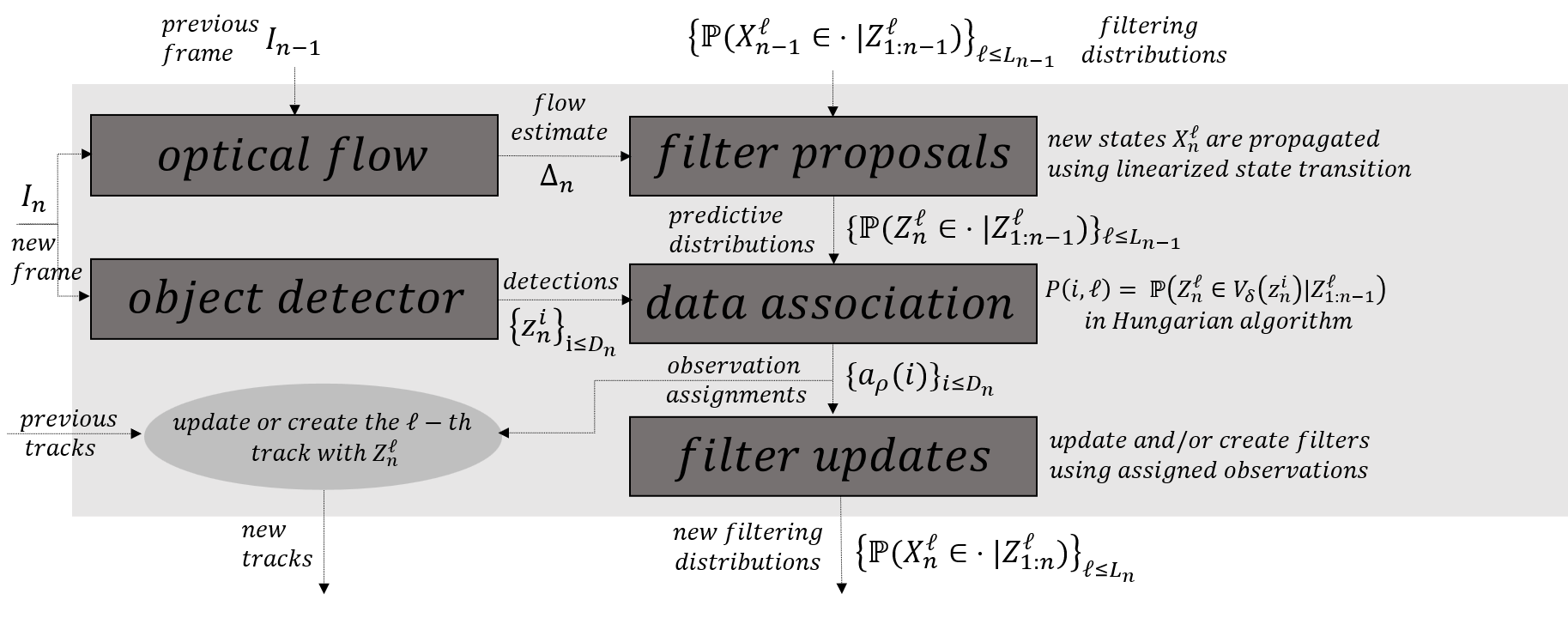
Visual representation of the tracking pipeline.
:::
## Counting
At the end of the video, the previous process returns a set of candidate
tracks. For counting purposes, we find that simple heuristics can be further
applied to filter out tracks that do not follow actual objects. More
precisely, we observe that tracks of real objects usually contain more (i)
observations and (ii) streams of uninterrupted observations. Denote by $T_\ell
= \left\{n \in \mathbb{N} \mid \exists z \in \mathcal{D}_n, Z_n^{\ell} =
z\right\}$ all timesteps where the $\ell$-th object is observed. To discard
false counts according to (i) and (ii), we compute the moving average
$M_\ell^\kappa$ of $1_{T_\ell}$ using windows of size $\kappa$, i.e. the
sequence defined by $M_\ell^\kappa[n] = \frac{1}{\kappa} \sum_{k \in [\![n -
\kappa, n + \kappa]\!]} 1_{T_\ell}[k]$. We then build $T_\ell^\kappa =
\left\{n \in T_\ell \mid M_\ell^\kappa[n] > \nu\right\}$, and defining
$\mathcal{N} = \left\{\ell \mid |T_\ell^\kappa| > \tau\right\}$, the final
object count is $|\mathcal{N}|$. We choose $\nu = 0.6$ while $\kappa,\tau$ are
optimized for best count performance (see @sec-tau_kappa_appendix for a
more comprehensive study).
# Metrics for MOT-based counting
Counting in videos using embedded moving cameras is not a common task, and as
such it requires a specific evaluation protocol to understand and compare the
performance of competing methods. First, not all MOT metrics are relevant,
even if some do provide insights to assist evaluation of count performance.
Second, considering only raw counts on long videos gives little information on
which of the final counts effectively arise from well detected objects.
## Count-related MOT metrics
Popular MOT benchmarks usually report several sets of metrics such as ClearMOT
(@bernardin2008) or IDF1 (@RistaniSZCT16) which can account for
different components of tracking performance. Recently, (@luiten2020)
built the so-called HOTA metrics that allow separate evaluation of detection
and association using the Jaccard index. The following components of their
work are relevant to our task (we provide equation numbers in the original
paper for formal definitions).
### Detection
First, when considering all frames independently, traditional detection recall
($\mathsf{DetRe}$) and precision ($\mathsf{DetPr}$) can be computed to assess the capabilities
of the object detector. Denoting with $\mathsf{TP}_n$, $\mathsf{FP}_n$, $\mathsf{FN}_n$ the number of
true positive, false positive and false negative detections at frame $n$,
respectively, we define $\mathsf{TP} = \sum_n \mathsf{TP}_n$, $\mathsf{FP} = \sum_n \mathsf{FP}_n$ and $\mathsf{FN} =
\sum_n \mathsf{FN}_n$, then:
$$\mathsf{DetRe} = \frac{\mathsf{TP}}{\mathsf{TP} + \mathsf{FN}},$$
$$\mathsf{DetPr} = \frac{\mathsf{TP}}{\mathsf{TP} + \mathsf{FP}}.$$
In classical object detection, those metrics are the main target.
In our context, as the first step of the system, this framewise performance impacts the difficulty of counting.
However, we must keep in mind that these metrics are computed framewise and might not guarantee anything at a video scale.
The next points illustrate that remark.
1. If both $\mathsf{DetRe}$ and $\mathsf{DetPr}$ are very high, objects are detected at nearly all frames and most detections come from actual objects.
Therefore, robustness to missing observations is high, but even in this context computing associations may fail if camera movements are nontrivial.
2. For an ideal tracking algorithm which never counts individual objects twice and does not confuse separate objects in a video, a detector capturing each object for only one frame could theoretically be used.
Thus, low $\mathsf{DetRe}$ could theoretically be compensated with robust tracking.
3. If our approach can rule out faulty tracks which do not follow actual objects, then good counts can still be obtained using a detector generating many false positives.
Again, this suggests that low $\mathsf{DetPr}$ may allow decent counting performance.
### Association
HOTA association metrics are built to measure tracking performance
irrespective of the detection capabilities, by comparing predicted tracks
against true object trajectories. In our experiments, we compute the
Association Recall ($\mathsf{AssRe}$) and the Association Precision ($\mathsf{AssPr}$).
Several intermediate quantities are necessary to introduce these final
metrics. Following @luiten2020, we denote with $\mathsf{prID}$ the ID of a predicted
track and $\mathsf{gtID}$ the ID of a ground truth track. Given $C$ all couples of
$\mathsf{prID}-\mathsf{gtID}$ found among the true positive detections, and $c \in C$ one of
these couples, $\mathsf{TPA}(c)$ is the number of frames where $\mathsf{prID}$ is also
associated with $\mathsf{gtID}$, $\mathsf{FPA}(c)$ is the number of frames where $\mathsf{prID}$ is
associated with another ground truth ID or with no ground truth ID, and
$\mathsf{FNA}(c)$ is the number of frames where $\mathsf{gtID}$ is associated with another
predicted ID or with no predicted ID. Then:
$$\mathsf{AssPr} = \frac{1}{\mathsf{TP}} \sum_{c \in C} \frac{\mathsf{TPA}(c)}{\mathsf{TPA}(c) + \mathsf{FPA}(c)},$$
$$\mathsf{AssRe} = \frac{1}{\mathsf{TP}} \sum_{c \in C} \frac{\mathsf{TPA}(c)}{\mathsf{TPA}(c) + \mathsf{FNA}(c)}.$$
See @luiten2020 (fig. 2) for a clear illustration of these quantities.
In brief, a low $\mathsf{AssPr}$ implies that several objects are often mingled into only one track, resulting in undercount.
A low $\mathsf{AssRe}$ implies that single objects are often associated with multiple tracks.
If no method is used to discard redundant tracks this results in overcount.
Conversely, association precision ($\mathsf{AssPr}$) measures how exclusive tracks are to each object (it decreases whenever a track covers multiple objects).
Again, it is useful to reconsider and illustrate the meaning of these metrics in the context of MOT-based counting.
Litter items are typically well separated on river banks, thus predicted tracks are not expected to interfere much.
This suggests that reaching high $\mathsf{AssPr}$ on our footage is not challenging.
Contrarily, $\mathsf{AssRe}$ is a direct measurement of the capability of the tracker to avoid producing multiple tracks despite missing detections and challenging motion.
A high $\mathsf{AssRe}$ therefore typically avoids multiple counts for the same object, which is a key aspect of our work.
Nonetheless, association metrics are only computed for predicted tracks which can effectively be matched with ground truth tracks.
Consequently, $\mathsf{AssRe}$ does not account for tracks predicted from streams of false positive detections generated by the detector (e.g.
arising from rocks, water reflections, etc).
Since such tracks induce false counts, a tracker which produces the fewest is better, but MOT metrics do not measure it.
## Count metrics
Denoting by $\mathsf{\hat{N}}$ and $\mathsf{N}$ the respective predicted and ground truth
counts for the validation material, the error $\mathsf{\hat{N}} - \mathsf{N}$ is misleading as
no information is provided on the quality of the predicted counts.
Additionally, results on the original validation footage do not measure the
statistical variability of the proposed estimators.
### Count decomposition
Define $i \in [\![1, \mathsf{N}]\!]$ and $j \in [\![1, \mathsf{\hat{N}}]\!]$ the labels of the
annotated ground truth tracks and the predicted tracks, respectively. At
evaluation, we assign each predicted track to either none or at most one
ground truth track, writing $j \rightarrow \emptyset$ or $j \rightarrow i$ for
the corresponding assignments. The association is made whenever a predicted
track $i$ overlaps with a ground truth track $j$ at any frame, i.e. for a
given frame a detection in $i$ is within a threshold $\alpha$ of an object in
$j$. We compute metrics for 20 values of $\alpha \in [0.05 \alpha_{max}, 0.95
\alpha_{max}]$, with $\alpha_{max} = 0.1 \sqrt{w^2 + h^2}$, then average the
results, which is the default method in HOTA to combine results at different
thresholds. We keep this default solution, in particular because our results
are very consistent accross different thresholds in that range (we only
observe a slight decrease in performance for $\alpha = \alpha_{max}$, where
occasional false detections probably start to lie below the threshold).
Denote $A_i = \{j \in [\![1, \mathsf{\hat{N}}]\!] \mid j \rightarrow i\}$ the set of predicted tracks assigned to the $i$-th ground truth track.
We define:
1. $\mathsf{\hat{N}_{true}} = \sum_{i=1}^{\mathsf{N}} 1_{|A_i| > 0}$ the number of ground truth objects successfully counted.
2. $\mathsf{\hat{N}_{red}} = \sum_{i=1}^{\mathsf{N}} |A_i| - \mathsf{\hat{N}_{true}}$ the number of redundant counts per ground truth object.
3. $\mathsf{\hat{N}_{mis}} = \mathsf{N} - \mathsf{\hat{N}_{true}}$ the number of ground truth objects that are never effectively counted.
4. $\mathsf{\hat{N}_{false}} = \sum_{j=1}^{\mathsf{\hat{N}}} 1_{j \rightarrow \emptyset}$ the number of counts which cannot be associated with any ground truth object and are therefore considered as false counts.
Using these metrics provides a much better understanding of $\mathsf{\hat{N}}$ as
$$
\mathsf{\hat{N}} = \mathsf{\hat{N}_{true}} + \mathsf{\hat{N}_{red}} + \mathsf{\hat{N}_{false}},
$$
while $\mathsf{\hat{N}_{mis}}$ completely summarises the number of undetected objects.
Conveniently, the quantities can be used to define the count precision ($\mathsf{CountPR}$) and count recall ($\mathsf{CountRe}$) as follows:
$$
\mathsf{CountPR} = \frac{\mathsf{\hat{N}_{true}}}{\mathsf{\hat{N}_{true}} + \mathsf{\hat{N}_{red}} + \mathsf{\hat{N}_{false}}},
$$
$$
\mathsf{CountRe} = \frac{\mathsf{\hat{N}_{true}}}{\mathsf{\hat{N}_{true}} + \mathsf{\hat{N}_{mis}}},
$$
which provide good summaries for the overall count quality, letting aside the tracking performance.
Note that these metrics and the associated decomposition are only defined if
the previous assignment between predicted and ground truth tracks can be
obtained. In our case, predicted tracks never overlap with several ground
truth tracks (because true objects are well separated), and therefore this
assignment is straightforward. More involved metrics have been studied at the
trajectory level (see for example @garcia2020 and the references
therein), though not specifically tailored to the restricted task of counting.
For more complicated data, an adaptation of such contributions into proper
counting metrics could be valuable.
### Statistics
Since the original validation set comprises only a few unequally long videos,
only absolute results are available. Splitting the original sequences into
shorter independent sequences of equal length allows to compute basic
statistics. For any quantity $\mathsf{\hat{N}}_\bullet$ defined above, we provide
$\hat{\sigma}_{\mathsf{\hat{N}}_\bullet}$ the associated empirical standard deviations
computed on the set of short sequences.
# Experiments
We denote by $S_1$, $S_2$ and $S_3$ the three river sections of the evaluation material and split the associated footage into independent segments of 30 seconds. We further divide this material into two distinct validation (6min30) and test (7min) splits.
To demonstrate the benefits of our work, we select two multi-object trackers
and build competing counting systems from them. Our first choice is SORT
@Bewley2016, which relies on Kalman filtering with velocity updated using the
latest past estimates of object positions. Similar to our system, it only
relies on image supervision for training, and though DeepSORT
(@Wojke2018) is a more recent alternative with better performance, the
associated deep appearance network cannot be used without additional video
annotations. FairMOT (@Zhanga), a more recent alternative, is similarly
intended for use with video supervision but allows self-supervised training
using only an image dataset. Built as a new baseline for MOT, it combines
linear constant-velocity Kalman filtering with visual features computed by an
additional network branch and extracted at the position of the estimated
object centers, as introduced in CenterTrack (@zhou2020). We choose
FairMOT to compare our method to a solution based on deep visual feature
extraction.
Similar to our work, FairMOT uses CenterNet for the detection part and the
latter is therefore trained as in @sec-detector_training. We train it using
hyperparameters from the original paper. The detection outputs are then shared
between all counting methods, allowing fair comparison of counting performance
given a fixed object detector. We run all experiments at 12fps, an
intermediate framerate to capture all objects while reducing the computational
burden.
## Detection
In the following section, we present the performance of the trained detector.
Having annotated all frames of the evaluation videos, we directly compute
$\mathsf{DetRe}$ and $\mathsf{DetPr}$ on those instead of a test split of the image dataset
used for training. This allows realistic assessment of the detection quality
of our system on true videos that may include blurry frames or artifacts
caused by strong motion. We observe low $\mathsf{DetRe}$, suggesting that objects are
only captured on a fraction of the frames they appear on. To better focus on
count performance in the next sections, we remove segments that do not
generate any correct detection: performance on the remaining footage is
increased and given by $\mathsf{DetRe}^{*}$ and $\mathsf{DetPr}^{*}$.
```{python}
from IPython.display import display
import pandas as pd

fps = 12
fps = f'{fps}fps'

split = 'test'

long_segments_names = ['part_1_1',
                    'part_1_2',
                    'part_2',
                    'part_3']

indices_test = [0,7,9,13]
indices_val = [0,9,10,14]
indices_det = [0,17,24,38]

alpha_type = '___50'

def set_split(split):

    if split == 'val':
        indices = indices_val
    elif split == 'test':
        indices = indices_test
    gt_dir_short = f'TrackEval/data/gt/surfrider_short_segments_{fps}'
    eval_dir_short = f'TrackEval/data/trackers/surfrider_short_segments_{fps}'
    if split is not None:
        gt_dir_short += f'_{split}'
        eval_dir_short += f'_{split}'
    gt_dir_short += '/surfrider-test'
    return indices, eval_dir_short, gt_dir_short

indices, eval_dir_short, gt_dir_short = set_split(split)

def get_det_values(index_start=0, index_stop=-1):

    results_for_det = pd.read_csv(os.path.join(f'TrackEval/data/trackers/surfrider_short_segments_{fps}','surfrider-test','ours_EKF_1_kappa_1_tau_0','pedestrian_detailed.csv'))
    results_det = results_for_det.loc[:,[f'DetRe{alpha_type}',f'DetPr{alpha_type}', f'HOTA_TP{alpha_type}',f'HOTA_FN{alpha_type}',f'HOTA_FP{alpha_type}']].iloc[index_start:index_stop]
    results_det.columns = ['hota_det_re','hota_det_pr','hota_det_tp','hota_det_fn','hota_det_fp']
    hota_det_re = results_det['hota_det_re']
    hota_det_pr = results_det['hota_det_pr']
    hota_det_tp = results_det['hota_det_tp']
    hota_det_fn = results_det['hota_det_fn']
    hota_det_fp = results_det['hota_det_fp']

    denom_hota_det_re = hota_det_tp + hota_det_fn
    denom_hota_det_pr = hota_det_tp + hota_det_fp

    hota_det_re_cb = (hota_det_re * denom_hota_det_re).sum() / denom_hota_det_re.sum()
    hota_det_pr_cb = (hota_det_pr * denom_hota_det_pr).sum() / denom_hota_det_pr.sum()

    return [f'{100*hota_det_re_cb:.1f}', f'{100*hota_det_pr_cb:.1f}']

def get_table_det():

    table_values = [get_det_values(index_start, index_stop) for (index_start, index_stop) in zip(indices_det[:-1],indices_det[1:])]
    table_values.append(get_det_values())
    return pd.DataFrame(table_values)

table_det = get_table_det()
table_det.columns = ['DetRe*','DetPr*']
table_det.index = ['S1','S2','S3','All']
display(table_det)
```
## Counts
To fairly compare the three solutions, we calibrate the hyperparameters of our
postprocessing block on the validation split and keep the values that minimize
the overall count error $\mathsf{\hat{N}}$ for each of them separately (see
@sec-tau_kappa_appendix for more information). All methods are found to work optimally at $\kappa = 7$, but our solution requires $\tau = 8$ instead of $\tau = 9$ for other solutions: this lower level of thresholding suggests that raw output of our tracking system is more reliable.
We report results using the count-related tracking metrics and count decompositions defined in the previous section. To provide a clear but thorough summary of the performance, we report $\mathsf{AssRe}$, $\mathsf{CountRe}$ and $\mathsf{CountPR}$ as tabled values (the first gives a simple overview of the quality of the predicted tacks while the latter two concisely summarise the count performance). For a more detailed visualisation of the different types of errors, we plot the count error decomposition for all sequences in a separate graph. Note that across all videos and all methods, we find $\mathsf{AssPr}$ between 98.6 and 99.2 which shows that this application context is unconcerned with tracks spanning multiple ground truth objects, therefore we do not conduct a more detailed interpretation of $\mathsf{AssPr}$ values.
First, the higher values of AssRe confirm the robustness of our solution in assigning consistent tracks to individual objects. This is directly reflected into the count precision performance - with an overall value of $\mathsf{CountPR}$ 17.6 points higher than the next best method (SORT) - or even more so in the complete disappearance of orange (redundant) counts in the graph. A key aspect is that these improvements are not counteracted by a lower $\mathsf{CountRe}$: on the contrary, our tracker, which is more stable, also captures more object (albeit still missing most of them, with a $\mathsf{CountRe}$ below 50%). Note finally, that the strongest improvements are obtained for sequence 2 which is also the part with the strongest motion.
```{python}
def get_summary(results, index_start=0, index_stop=-1):

    results = results.loc[:,[f'Correct_IDs{alpha_type}',f'Redundant_IDs{alpha_type}',f'False_IDs{alpha_type}',f'Missing_IDs{alpha_type}',f'Fused_IDs{alpha_type}', f'GT_IDs',f'HOTA_TP{alpha_type}',f'AssRe{alpha_type}']].iloc[index_start:index_stop]

    results.columns = ['correct','redundant','false','missing','mingled','gt','hota_tp','ass_re']

    ass_re = results['ass_re']
    hota_tp = results['hota_tp']


    ass_re_cb = (ass_re * hota_tp).sum() / hota_tp.sum()

    correct = results['correct']
    redundant = results['redundant']
    false = results['false']
    missing = results['missing']

    summary = dict()
    summary['ass_re_cb'] = f'{100*ass_re_cb:.1f}'


    count_re = correct.sum() / (correct + missing).sum()
    summary['count_re_cb'] = f'{100*count_re:.1f}'

    count_re_std = (correct / (correct + missing)).std()
    summary['count_re_std'] = f'{100*np.nan_to_num(count_re_std):.1f}'

    count_pr = correct.sum() / (correct + false + redundant).sum()
    summary['count_pr_cb'] = f'{100*count_pr:.1f}'

    count_pr_std = (correct / (correct + false + redundant)).std()
    summary['count_pr_std'] = f'{100*np.nan_to_num(count_pr_std):.1f}'

    return summary


def get_summaries(results, sequence_names):

    summaries = dict()

    for (sequence_name, index_start, index_stop) in zip(sequence_names, indices[:-1], indices[1:]):

        summaries[sequence_name] = get_summary(results, index_start, index_stop)

    summaries['All'] = get_summary(results)

    return summaries


summaries = []
method_names = ['fairmot_kappa_7_tau_9', 'sort_kappa_7_tau_9','ours_EKF_1_kappa_7_tau_8']
pretty_method_names = ['FairMOT','SORT','Ours']
for tracker_name in method_names:
    results = pd.read_csv(os.path.join(eval_dir_short,'surfrider-test',tracker_name,'pedestrian_detailed.csv'))
    sequence_names = ['S1','S2','S3']
    summaries.append(pd.DataFrame(get_summaries(results, sequence_names)).T)


fairmot_star, sort, ours = summaries

rows = ['fairmot_kappa_7_tau_9','sort_kappa_7_tau_9','ours_EKF_1_kappa_7_tau_8']
columns = ['ass_re','count_re', 'count_re_std', 'count_pr', 'count_pr_std']

for summary in summaries:
    summary.columns = columns

results_S1 = pd.DataFrame([summary.iloc[0] for summary in summaries])
results_S1.index = method_names

results_S2 = pd.DataFrame([summary.iloc[1] for summary in summaries])
results_S2.index = method_names

results_S3 = pd.DataFrame([summary.iloc[2] for summary in summaries])
results_S3.index = method_names

results_All = pd.DataFrame([summary.iloc[3] for summary in summaries])
results_All.index = method_names

results = [results_S1, results_S2, results_S3, results_All]
column_names = [
    "AssRe",
    r"CountRe",
    r"σ(CountRe)",
    r"CountPr",
    r"σ(CountPr)"]
row_names = ["FairMOT", "Sort", "Ours"]

for result in results:
    result.columns = column_names
    result.index = row_names

results_S1
```
```{python}
results_S2
```
```{python}
results_S3
```
```{python}
results_All
```
#### Detailed results on individual segments
```{python}
set_split('test')
fig, axes = plt.subplots(1,3, figsize=(30,10), sharey=True)
for ax, title, tracker_name in zip(axes, pretty_method_names,  method_names):
    results = pd.read_csv(os.path.join(eval_dir_short,'surfrider-test',tracker_name,'pedestrian_detailed.csv'))
    results = results.loc[:,[f'Redundant_IDs{alpha_type}',f'False_IDs{alpha_type}',f'Missing_IDs{alpha_type}']].iloc[:-1]
    results.columns = ['redundant', 'false', 'missing']
    results.loc[:,'missing'] = - results.loc[:,'missing']
    results.columns = ['$\hat{\mathsf{N}}_{red}$', '$\hat{\mathsf{N}}_{false}$', '$-\hat{\mathsf{N}}_{mis}$']
    results.plot(ax = ax, kind='bar', stacked=True, color=['orange', 'red', 'black'], title=title, xlabel='Sequence nb')
```
# Practical impact and future goals
We successfully tackled video object counting on river banks, in particular issues which could be addressed independently of detection quality.
Moreover the methodology developed to assess count quality enables us to precisely highlight the challenges that pertain to video object counting on river banks.
Conducted in coordination with Surfrider Foundation Europe, an NGO specialized on water preservation, our work marks an important milestone in a broader campaign for macrolitter monitoring and is already being used in a production version of a monitoring system.
That said, large amounts of litter items are still not detected.
Solving this problem is largely a question of augmenting the object detector training dataset through crowdsourced images.
A [specific annotation platform](https://www.trashroulette.com) is online, thus the amount of annotated images is expected to continuously increase, while training is provided to volunteers collecting data on the field to ensure data quality.
Finally, several expeditions on different rivers are already underway and new video footage is expected to be annotated in the near future for better evaluation.
All data is made freely available.
Future goals include downsizing the algorithm, a possibility given the architectural simplicity of anchor-free detection and the relatively low computational complexity of EKF.
In a citizen science perspective, a fully embedded version for portable devices will allow a larger deployment.
The resulting field data will help better understand litter origin, allowing to model and predict litter density in non surveyed areas.
Correlations between macro litter density and environmental parameters will be studied (e.g., population density, catchment size, land use and hydromorphology).
Finally, our work naturally benefits any extension of macrolitter monitoring in other areas (urban, coastal, etc) that may rely on a similar setup of moving cameras.
# Supplements
## Details on the image dataset {#sec-image_dataset_appendix}
### Categories
In this work, we do not seek to precisely predict the proportions of the
different types of counted litter. However, we build our dataset to allow
classification tasks. Though litter classifications built by experts already
exist, most are based on semantic rather than visual features and do not
particularly consider the problem of class imbalance, which makes statistical
learning more delicate. In conjunction with water pollution experts, we
therefore define a custom macrolitter taxonomy which balances annotation ease
and pragmatic decisions for computer vision applications. This classification,
depicted in @fig-trash-categories-image can be understood as follows.
1. We define a set of frequently observed classes that annotateors can choose from, divided into:
- Classes for rigid and easily recognisable items which are often observed and have definite shapes
- Classes for fragmented objects which are often found along river banks but whose aspects are more varied
2. We define two supplementary categories used whenever the annotater cannot classify the item they are observing in an image using classes given in 1.
- A first category is used whenever the item is clearly identifiable but its class is not proposed.
This will ensure that our classification can be improved in the future, as images with items in this category will be checked regularly to decide whether a new class needs to be created.
- Another category is used whenever the annotater does not understand the item they are seeing.
Images containing items denoted as such will not be used for applications involving classification.
::: {#fig-trash-categories-image}
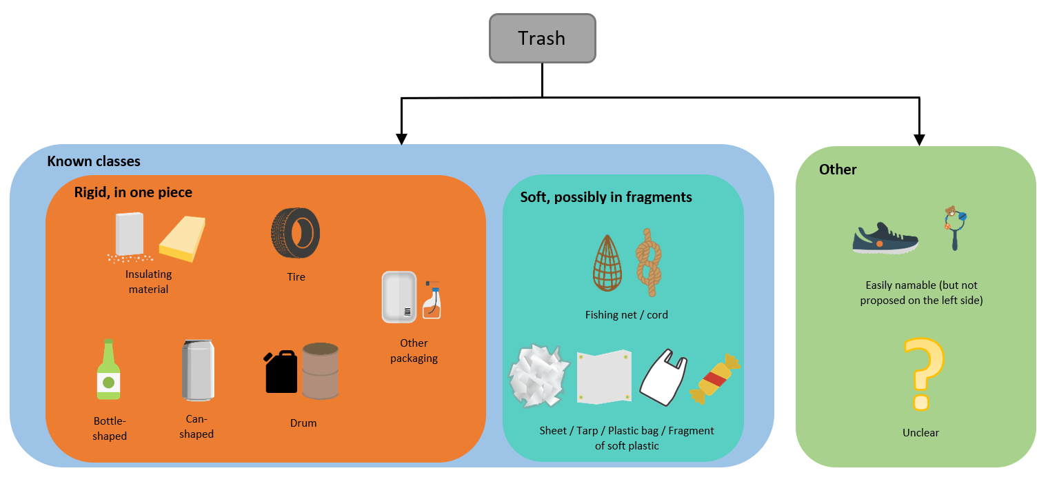
Trash categories defined to facilitate porting to a counting system that allows trash identification
:::
## Details on the evaluation videos {#sec-video-dataset-appendix}
### River segments
In this section, we provide further details on the evaluation material.
@fig-river-sections shows the setup and positioning of the three river
segments $S_1$, $S_2$ and $S_3$ used to evaluate the methods. The segments
differ in the following aspects.
- Segment 1: Medium current, high and dense vegetation not obstructing vision of the right riverbank from watercrafts, extra objects installed before the field experiment.
- Segment 2: High current, low and dense vegetation obstructing vision of the right riverbank from watercrafts.
- Segment 3: Medium current, high and little vegetation not obstructing vision of the left riverbank from watercrafts.
::: {#fig-river-sections}
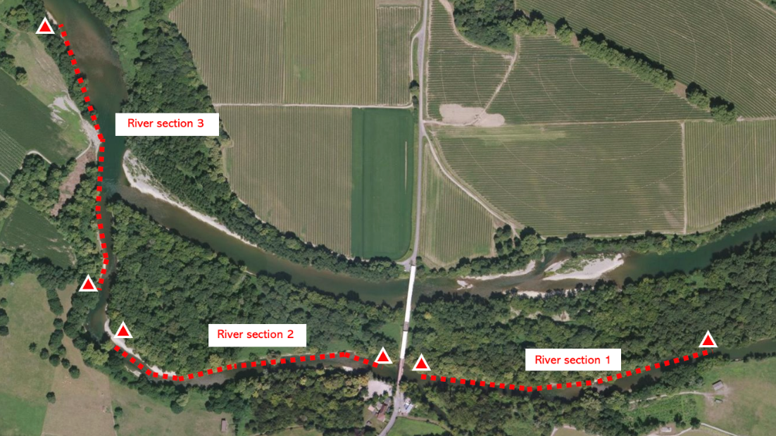
Aerial view of the three river segments of the evaluation material
:::
#### Track annotation protocol
To annotate tracks on the evaluation sequences, we used the online tool "CVAT" which allows to locate bounding boxes on video frames and propagate them in time.
The following items provide further details on the exact annotation process.
- Object tracks start whenever a litter item becomes fully visible and identifiable by the naked eye.
- Positions and sizes of objects are given at nearly every second of the video with automatic interpolation for frames in-between: this yields clean tracks with precise positions at 24fps.
- We do not provide inferred locations when an object is fully occluded, but tracks restart with the same identity whenever the object becomes visible again.
- Tracks stop whenever an object becomes indistinguishable and will not reappear again.
## Implementation details for the tracking module {#sec-tracking_module_appendix}
### Covariance matrices for state and observation noises {#sec-covariance_matrices}
In our state space model, $Q$ models the noise associated with the movement
model we posit in @sec-bayesian_tracking involving optical flow estimates,
while $R$ models the noise associated with the observation of the true
position via our object detector. An attempt to estimate the diagonal values
of these matrices was the following.
- To estimate $R$, we computed a mean $L_2$ error between the known positions of objects and the associated predictions by the object detector, for images in our training dataset.
- To estimate $Q$, we built a small synthetic dataset of consecutive frames taken from videos, where positions of objects in two consecutive frames are known.
We computed a mean $L_2$ error between the known positions in the second frame and the positions estimated by shifting the positions in the first frame with the estimated optical flow values.
This led to $R_{00} = R_{11} = 1.1$, $Q_{00} = 4.7$ and $Q_{11} = 0.9$, for grids of dimensions $\lfloor w/p\rfloor \times \lfloor h/p\rfloor = 480 \times 270$.
All other coefficients were not estimated and supposed to be 0.
An important remark is that though we use these values in practice, we found that tracking results are largely unaffected by small variations of $R$ and $Q$.
As long as values are meaningful relative to the image dimensions and the size of the objects, most noise levels show relatively similar performance.
### Influence of $\tau$ and $\kappa$ {#sec-tau_kappa_appendix}
An understanding of $\kappa$, $\tau$ and $\nu$ can be stated as follows.
For any track, given a value for $\kappa$ and $\nu$, an observation at time $n$ is only kept if there are also $\nu \cdot \kappa$ observations in the temporal window of size $\kappa$ that surrounds $n$ (windows are centered around $n$ except at the start and end of the track).
The track is only counted if the remaining number of observations is strictly higher than $\tau$.
At a given $\nu > 0.5$, $\kappa$ and $\tau$ should ideally be chosen to jointly decrease $\mathsf{\hat{N}_{false}}$ and $\mathsf{\hat{N}_{red}}$ as much as possible without increasing $\mathsf{\hat{N}_{mis}}$ (true objects become uncounted if tracks are discarded too easily).
In the following code cell, we plot the error decomposition of the counts for several values of $\kappa$ and $\tau$ with $\nu=0.6$ for the outputs of the three different trackers. We choose $\nu = 0.7$ and compute the optimal point as the one which minimizes the overall count error $\mathsf{\hat{N}} (= \mathsf{\hat{N}_{mis}} + \mathsf{\hat{N}_{red}} + \mathsf{\hat{N}_{false}})$.
```{python}
set_split('val')

params = {'legend.fontsize': 'x-large',
         'axes.labelsize': 'x-large',
         'axes.titlesize':'x-large',
         'xtick.labelsize':'x-large',
         'ytick.labelsize':'x-large'}
plt.rcParams.update(params)


def hyperparameters(method_name, pretty_method_name):
    tau_values = [i for i in range(1,10)]
    kappa_values = [1,3,5,7]
    fig, (ax0, ax1, ax2) = plt.subplots(3,1)
    pretty_names=[f'$\kappa={kappa}$' for kappa in kappa_values]
    n_count = {}
    for kappa, pretty_name in zip(kappa_values, pretty_names):
        tracker_names = [f'{method_name}_kappa_{kappa}_tau_{tau}' for tau in tau_values]
        all_results = {tracker_name: pd.read_csv(os.path.join(eval_dir_short,'surfrider-test',tracker_name,'pedestrian_detailed.csv')).iloc[:-1] for tracker_name in tracker_names}

        n_missing = []
        n_false = []
        n_redundant = []
        for tracker_name, tracker_results in all_results.items():
            missing = (tracker_results['GT_IDs'].sum() - tracker_results['Correct_IDs___50'].sum())
            false = tracker_results['False_IDs___50'].sum()
            redundant = tracker_results['Redundant_IDs___50'].sum()

            n_missing.append(missing)
            n_false.append(false)
            n_redundant.append(redundant)
            n_count[tracker_name] = missing + false + redundant


        ax0.scatter(tau_values, n_missing)
        ax0.plot(tau_values, n_missing, label=pretty_name, linestyle='dashed')
        # ax0.set_xlabel('$\\tau$')
        ax0.set_ylabel('$N_{mis}$')

        ax1.scatter(tau_values, n_false)
        ax1.plot(tau_values, n_false, linestyle='dashed')

        # ax1.set_xlabel('$\\tau$')
        ax1.set_ylabel('$N_{false}$')

        ax2.scatter(tau_values, n_redundant)
        ax2.plot(tau_values, n_redundant, linestyle='dashed')
        ax2.set_xlabel('$\\tau$')
        ax2.set_ylabel('$N_{red}$')


    best_value = np.inf
    best_key = ''

    for k, v in n_count.items():
        if v < best_value: best_key = k
        best_value = v
    best_key = best_key.split('kappa')[1]
    best_kappa = int(best_key.split('_')[1])
    best_tau = int(best_key.split('_')[-1])
    print(f'Best parameters for {pretty_method_name}: (kappa, tau) = ({best_kappa}, {best_tau})')
    handles, labels = ax0.get_legend_handles_labels()
    fig.legend(handles, labels, loc='upper right')
    plt.autoscale(True)

    plt.tight_layout()
    plt.show()
    plt.close()

for method_name, pretty_method_name in zip(method_names, pretty_method_names):
    hyperparameters(method_name.split('kappa')[0][:-1], pretty_method_name)
```
## Bayesian filtering {#sec-bayesian_filtering}
Considering a state space model with $(X_k, Z_k)_{k \geq 0}$ the random processes for the states and observations, respectively, the filtering recursions are given by:
- The predict step: $p(x_{k+1}|z_{1:k}) = \int p(x_{k+1}|x_k)p(x_k|z_{1:k})\mathrm{d}x_k.$
- The update step: $p(x_{k+1}|z_{1:k+1}) \propto p(z_{k+1} | x_{k+1})p(x_{k+1}|z_{1:k}).$
The recursions are intractable in most cases, but when the model is linear and Gaussian, i.e. such that:
$$X_{k} = A_kX_{k-1} + a_k + \eta_k$$
$$Z_{k} = B_kX_{k} + b_k + \epsilon_k$$
with $\eta_k \sim \mathcal{N}(0,Q_k)$ and $\epsilon_k \sim \mathcal{N}(0,R_k)$, then the distribution of $X_k$ given $Z_{1:k}$ is a Gaussian $\mathcal{N}(\mu_k,\Sigma_k)$ following:
- $\mu_{k|k-1} = A_k\mu_{k-1} + a_k$ and $\Sigma_{k|k-1} = A_k \Sigma_{k-1} A_k^T + Q_k$ (Kalman predict step),
- $\mu_{k} = \mu_{k|k-1} + K_k\left[Z_k - (B_k\mu_{k|k-1} + b_k)\right]$ and $\Sigma_{k} = (I - K_kB_k)\Sigma_{k|k-1}$ (Kalman update step),
where $K_k = \Sigma_{k|k-1}B_k^T(B_k \Sigma_{k|k-1} B_k^T + R_k)^{-1}$.
In the case of the linearized model in @sec-state_space_model, EKF consists in applying these updates with:
$$A_k = (I + \partial_X\Delta_k(\lfloor \mu_{k-1} \rfloor),$$
$$a_k = \Delta_k(\lfloor \mu_{k-1} \rfloor) - \partial_X\Delta_k(\lfloor \mu_{k-1} \rfloor)\mu_{k-1},$$
$$Q_k = Q, R_k = R,$$
$$B_k = I, b_k = 0.$$
## Computing the confidence regions {#sec-confidence_regions_appendix}
In words, $P(i,\ell)$ is the mass in $V_\delta(z_n^i) \subset \mathbb{R}^2$ of the
probability distribution of $Z_n^\ell$ given $Z_{1:n-1}^\ell$. It is related
to the filtering distribution at the previous timestep via
$$
p(z_n | z_{1:n-1}) = \int \int p(z_n | x_n) p(x_n | x_{n-1}) p(x_{n-1} | z_{1:n-1}) \mathrm{d} x_{n} \mathrm{d} x_{n-1}
$$
When using EKF, this distribution is a multivariate Gaussian whose moments can be analytically obtained from the filtering mean and variance and the parameters of the linear model, i.e.
$$
\mathbb{E} \left[Z_n^\ell | Z_{1:n-1}^\ell \right] = B_k (A_k \mu_{k-1} + a_k) + b_k
$$
and
$$
\mathbb{V} \left[Z_n^\ell | Z_{1:n-1}^\ell \right] = B_k (A_k \Sigma_k A_k^T + Q_k) B_k^T + R_k
$$
following the previously introduced notation. Note that given the values of $A_k, B_k, a_k, b_k$ in our model these equations are simplified in practice, e.g. $B_k = I, b_k = 0$ and $A_k \mu_{k-1} + a_k = \mu_{k-1} + \Delta_k(\lfloor \mu_{k-1} \rfloor)$.
In $\mathbb{R}^2$, values of the cumulative distribution function (cdf) of a multivariate Gaussian distribution are easy to compute.
Denote with $F_n^\ell$ the cdf of $\mathbb{L}_n^\ell$.
If $V_\delta(z)$ is a squared neighborhood of size $\delta$ and centered on $z=(x,y) \in \mathbb{R}^2$, then, denoting with $\mathbb{L}_n^\ell$ the distribution of $Z_n^\ell$ given $Z_{1:n-1}^\ell$:
$$
\mathbb{L}_n^{\ell}(V_\delta(z)) = F_n^\ell(x+\delta,y+\delta) + F_n^\ell(x-\delta,y-\delta) - \left[F_n^\ell(x+\delta,y-\delta) + F_n^\ell(x-\delta,y+\delta)\right]
$$
This allows easy computation of $P(i,\ell) = \mathbb{L}_n^\ell(V_\delta(z_n^i))$.
### Impact of the filtering algorithm {#sec-impact-algorithm-appendix}
An advantage of the data association method proposed in @sec-data_association
is that it is very generic and does not constrain the tracking solution to any
particular choice of filtering algorithm. As for EKF, UKF implementations are
already available to compute the distribution of $Z_k$ given $Z_{1:k-1}$ and
the corresponding confidence regions (see @sec-tracking_module_appendix above). We propose a solution to compute
this distribution when SMC is used, and performance comparisons between the
EKF, UKF and SMC versions of our trackers are discussed.
### SMC-based tracking
Denote $\mathbb{Q}_k$ the filtering distribution (ie. that of $Z_k$ given $X_{1:k}$) for the HMM $(X_k,Z_k)_{k \geq 1}$ (omitting the dependency on the observations for notation ease).
Using a set of samples $\{X_k^i\}_{1 \leq i \leq N}$ and importance weights $\{w_k^i\}_{1 \leq i \leq N}$, SMC methods build an approximation of the following form:
$$
\widehat{\mathbb{Q}}^{SMC}_k(\mathrm{d} x_k) = \sum_{i=1}^N w_k^i \delta_{X_k^i}(\mathrm{d} x_k) \,.
$$
Contrary to EKF and UKF, the distribution $\mathbb{L}_k$ of $Z_k$ given $Z_{1:k-1}$ is not directly available but can be obtained via an additional Monte Carlo sampling step.
Marginalizing over $(X_{k-1}$, $X_k)$ and using the conditional independence properties of HMMs, we decompose $\mathbb{L}_k$ using the conditional state transition $\mathbb{M}_k(x,\mathrm{d} x')$ and the likelihood of $Z_k$ given $X_k$, denoted by $\mathbb{G}_k(x, \mathrm{d} z)$:
$$
\mathbb{L}_k(\mathrm{d} z_k) = \int \int \mathbb{G}_k(x_k, \mathrm{d} z_k)\mathbb{M}_k(x_{k-1}, \mathrm{d} x_k)\mathbb{Q}_{k-1}(\mathrm{d} x_{k-1}) \,.
$$
Replacing $\mathbb{Q}_{k-1}$ with $\widehat{\mathbb{Q}}^{SMC}_{k-1}$ into the previous equation yields
$$
\widehat{\mathbb{L}}^{SMC}_k(\mathrm{d} z_k) = \sum_{k=1}^N w_k^i \int \mathbb{G}_k(x_k,\mathrm{d} z_k) \mathbb{M}_k(X_{k-1}^i, \mathrm{d} x_k) \,.
$$
In our model, the state transition is Gaussian and therefore easy to sample from.
Thus an approximated predictive distribution $\widehat{\mathbb{L}}_k$ can be obtained using Monte Carlo estimates built from random samples $\{X_k^{i,j}\}_{1 \leq i \leq N}^{1 \leq j \leq M}$ drawn from $\mathbb{M}_k(X_{k-1}^i, \mathrm{d} x_k)$.
This leads to
$$
\widehat{\mathbb{L}}_k(\mathrm{d} z_k) = \sum_{i=1}^N \sum_{j=1}^M w_k^i \mathbb{G}_k(X_k^{i,j},\mathrm{d} z_k) \,.
$$
Since the observation likelihood is also Gaussian, $\widehat{\mathbb{L}}_k$ is
a Gaussian mixture, thus values of $\widehat{\mathbb{L}}_k(\mathsf{A})$ for
any $\mathsf{A} \subset \mathbb{R}^2$ can be computed by applying the tools
from @sec-confidence_regions_appendix to all mixture components.
Similar to EKF and UKF, this approximated predictive distribution is used to
recover object identities via $\widehat{\mathbb{L}}_n^{\ell}(V_\delta(z_n^i))$
computed for all incoming detections $\mathcal{D}_n = \{z_n^i\}_{1 \leq i \leq D_n}$ and each of the $1 \leq \ell \leq L_n$ filters, where $\widehat{\mathbb{L}}_n^{\ell}$ is the predictive distribution associated with the $\ell$-th filter.
### Performance comparison
In theory, sampling-based methods like UKF and SMC are better suited for
nonlinear state space models like the one we propose in @sec-state_space_model.
However, we observe very few differences in count results when upgrading from EKF to UKF to SMC.
In practise, there is no difference at all between our EKF and UKF implementations, which show strictly identical values for $\mathsf{\hat{N}_{true}}$, $\mathsf{\hat{N}_{false}}$ and $\mathsf{\hat{N}_{red}}$.
For the SMC version, values for $\mathsf{\hat{N}_{false}}$ and $\mathsf{\hat{N}_{red}}$ improve by a very small amount (2 and 1, respectively), but $\mathsf{\hat{N}_{mis}}$ is slightly worse (one more object missed), and these results depend loosely on the number of samples used to approximate the filtering distributions and the number of samples for the Monte Carlo scheme.
Therefore, our motion estimates via the optical flow $\Delta_n$ prove very reliable in our application context, so much that EKF, though suboptimal, brings equivalent results.
This comforts us into keeping it as a faster and computationally simpler option.
That said, this conclusion might not hold in scenarios where camera motion is even stronger, which was our main motivation to develop a flexible tracking solution and to provide implementations of UKF and SMC versions.
This allows easier extension of our work to more challenging data.
# References {.unnumbered}
::: {#refs}
:::