::: {.content-hidden}
\(
\newcommand{\bbR}{\mathbb{R}}
\newcommand{\calA}{\mathcal{A}}
\newcommand{\calC}{\mathcal{C}}
\newcommand{\calD}{\mathcal{D}}
\newcommand{\calF}{\mathcal{F}}
\newcommand{\calL}{\mathcal{L}}
\newcommand{\calM}{\mathcal{M}}
\newcommand{\calO}{\mathcal{O}}
\newcommand{\calP}{\mathcal{P}}
\newcommand{\calQ}{\mathcal{Q}}
\newcommand{\calX}{\mathcal{X}}
\newcommand{\Os}{O^{\sharp}}
\newcommand{\pr}{\widehat{\text{pr}}}
\newcommand{\thn}{\widehat{\theta}_{n}}
\newcommand{\card}{\mathop{\mathrm{card}}}
\newcommand{\Class}{\mathop{\mathrm{Class}}}
\newcommand{\Corr}{\mathop{\mathrm{Corr}}}
\newcommand{\Dec}{\mathop{\mathrm{Dec}}}
\newcommand{\diag}{\mathop{\mathrm{diag}}}
\newcommand{\Enc}{\mathop{\mathrm{Enc}}}
\newcommand{\expit}{\mathop{\mathrm{expit}}}
\newcommand{\Gen}{\mathop{\mathrm{Gen}}}
\newcommand{\KL}{\mathop{\mathrm{KL}}}
\newcommand{\law}{\mathop{\mathrm{law}}}
\newcommand{\LB}{\mathop{\mathrm{LB}}}
\newcommand{\Unif}{\mathop{\mathrm{Unif}}}
\newcommand{\ReLU}{\mathop{\mathrm{ReLU}}}
\)
:::
> Asher Rubin walks out of the starosta's home and heads toward the market square. With evening, the sky has cleared, and now a million stars are shining, but their light is cold and brings down a frost upon the earth, upon Rohatyn. The first of this autumn. Rubin pulls his black wool coat tighter around him; tall and thin, he looks like a vertical line.
[@Tokarczuk, I(3)]
# Introduction
## Fiction as the original simulation
One of humanity's oldest creative endeavors, fiction represents an early form
of simulation. It extends the imaginative play where children create
scenarios, roles, or worlds that are not constrained by the rules of reality,
that is "childhood pretence" [@Carruthers] or "the make-believe games" of
children [@Walton]. Through stories, myths, and imagined worlds, humans
construct alternative realities to explore ideas, express emotions, and
reflect on their existence. By presenting hypothetical scenarios and posing
"what if things had been different" questions [@Pearl, page 34], fiction
empowers individuals to explore alternative histories, draw insights from the
experiences of others, and engage with possibilities that extend beyond the
confines of the physical world. At its core, fiction abstracts and
reconstructs elements of reality. An author selectively includes, exaggerates,
or omits aspects of the real world, creating models that serve their artistic
or thematic intentions. From Homer's *Odyssey* [@Jaccottet] to speculative
tales like Mary Shelley's *Frankenstein* [@Shelley], fiction mirrors the
complexities of human life, enabling readers to engaged with an imagined
reality that resonates with their own.
The relationship between fiction and reality has long been a subject of
debate. Plato, in his critique of art, viewed fiction as a mere imitation of
the physical world, itself a flawed reflection of the ideal "Forms". By this
reasoning, fiction is a "simulation of a simulation", twice removed from truth
[@Platon, Livre X]. Aristotle, by contrast, argued that fiction, through
"mimesis", the imitation of action and life, can illuminate universal truths
[@Aristote, Chapitres 1 à 5]. By abstracting from the particular, fiction
allows exploration of broader patterns and principles.
Following Aristotle's perspective, this tradition of creating and interacting
with imagined realities provides a natural foundation for distinguishing
scientific theories from scientific models [@Barberousse] and understanding
modern simulations. While they stem from the same drive to represent and
explore, scientific theories, scientific models and modern simulations
introduce a higher degree of mathematical rigor. Nevertheless, fiction
remains their conceptual ancestor, reminding us that the human impulse to
model and engage with alternate realities is as old as storytelling itself.
## From modern simulations to computer simulations {#sec-modern-computer-simulations}
The concept of modern simulations predates the modern era. Early instances
include mechanical devices like the Antikythera, a sophisticated analog
computer from the 2nd century BCE designed to simulate celestial movements
[and the MacGuffin chased by Indiana Jones in the 2024 installment of the
franchise, @Antikythera]. The emergence of mathematical models in the works of
Galileo and Newton introduced a new form of simulation, where equations were
used to predict physical phenomena with increasing precision. By the 18th
century, probabilistic experiments like Buffon's Needle, designed to
approximate the number $\pi$ [@Proofs, section 24], demonstrated the power of
simulating complex systems. However, the advent of computer simulations, as
we understand them today, began during World War II with the work of J.\ von
Neumann and S.\ Ulam [@metropolis1949monte].
While studying neutron behavior, they faced a challenge that was too complex
for theoretical analysis and too hazardous, time-consuming, and costly to
investigate experimentally. Fundamental properties (e.g., possible events and
their probabilities) and basic quantities (e.g., the average distance a
neutron would travel before colliding with an atomic nucleus, the likelihood
of absorption or reflection, and energy loss after collisions) were known, but
predicting the outcomes of entire event sequences was infeasible. To address
this challenge, they devised a method of generating random sequences step by
step using a computer, naming it "Monte Carlo" after the casino, a suggestion
by N.\ Metropolis. Statistical analysis of the data produced by repeatedly
applying this method provided sufficiently accurate solutions to better
understand nuclear chain reactions, a crucial aspect of designing atomic bombs
and later nuclear reactors. This breakthrough marked the birth of modern
computer simulations.
Today, computer simulations, henceforth referred to simply as *simulations*,
play a fundamental role in applied mathematics. Generally, conducting a
simulation involves running a computer program (a "simulator") designed to
represent a "system of interest" at a problem-dependent level of abstraction
(that is, with a specific degree of complexity) and collecting the numerical
output for analysis.
Examples of systems of interest are virtually limitless and highly diverse.
They can represent a real-world process in a holistic fashion, such as the
regular functioning of a person's heart at rest, or the medical trajectories
of a cohort of patients undergoing chemotherapy. Alternatively, in a more
focused fashion, they can consist of a hybrid pipeline that combines an
upstream real-world process with downstream data processing of intermediary
outputs, such as the estimation of peripheral oxygen saturation in a healthy
patient using a pulse oximeter. Regardless of the context, determining the
appropriate levels of abstraction and realism is always a significant
challenge.
Here, we focus on simulations used to evaluate the performance of statistical
procedures through simulation studies, as discussed by @MWC19 in their
excellent tutorial on the design and conduct of such studies. The interested
reader will find in their work a carefully curated list of books on simulation
methods in general and articles emphasizing rigor in specific aspects of
simulation studies. Specifically, we consider scenarios where a statistician,
interested in a real-world process, has developed an algorithm tailored to
learning a particular feature of that process from collected data and seeks to
assess the algorithm's performance through simulations.
Once the simulator is devised, the following process is repeated multiple
times. In each iteration, typically independently from previous iterations:
first, the simulator generates a synthetic data set of size $n$; second, the
algorithm is run on the generated data; third, the algorithm's output is
collected for further analysis. After completing these iterations, the next
step is to compare the outcome from one run to the algorithm's target. This is
made possible by the design of the simulator. Finally, the overall
performance of the algorithm is assessed by comparing all the results
collectively to the algorithm's target. Depending on the task, this evaluation
can involve assessing the algorithm's ability to well estimate its target, the
validity of the confidence regions it constructs for its target, the
algorithm's ability to detect whether its target lies within a specified null
domain (using an alternative domain as a reference), and more. This list is
far from exhaustive. The entire process can be repeated multiple times, for
example, to assess how the algorithm's performance depends on $n$.
However, in order to carry out these steps, the statistician must first devise
a simulator. This simulator should ideally generate synthetic data that
resemble the real-world data in a meaningful way, a goal that is often
difficult to achieve. So, how can one design a realistic simulator, and what
does "realistic simulator" even mean in this context? These are the central
questions we explore in this work.
## A probabilistic stance
We adopt a probabilistic framework to model the data collected by observing a
real-world process. Specifically, the data are represented as a random
variable $O^{n}$ ($O$ as in *observations*) drawn from a probability law
$P^{n}$ ($P$ as in *probability*). The law $P^{n}$ is assumed to belong to a
statistical model $\calM^{n}$ ($\calM$ as in *model*), which is the set of all
probability laws on the space $\calO^{n}$ where $O^{n}$ takes its values. This
model incorporates constraints that reflect known properties of the real-world
process and, where necessary, minimal assumptions about it.
The superscript $n$ indicates an amount of information. For example, in the
context of this study, $n$ typically represents the number of elementary
observations drawn independently from a law $P$ on $\calO$ and gathered in
$O^{n}$. In this case, $\calO^{n}$ corresponds to the Cartesian product $\calO
\times \cdots\times \calO$ (repeated $n$ times) and $P^{n}$ to the product law
$P^{\otimes n}$, with $O^{n}$ decomposing as $(O_{1}, \ldots, O_{n})$
The feature of interest is an element of a space $\calF$ (e.g., a subset of
the real line, or a set of functions). It is modeled as the value
$\Psi(P^{n})$ of a functional $\Psi:\calM^{n} \to \calF$ evaluated at $P^{n}$.
The algorithm developed to estimate this feature is modeled as a functional
$\calA : \calO^{n} \to \calF$. Training the algorithm involves applying
$\calA$ to the observed data $O^{n}$, resulting in the estimator
$\calA(O^{n})$ for the estimand $\Psi(P^{n})$.
We emphasize that we address the questions closing
@sec-modern-computer-simulations without focusing on the specific nature of
the functional of interest $\Psi$: how can one design a realistic simulator,
and what does "realistic simulator" even mean in this context?
## Draw me a simulator {#sec-draw-me-a-model}
When constructing simulators, there is a spectrum of approaches, varying in
complexity and flexibility. At one end of the spectrum, simulators are built
upon relatively simple parametric models. While these models are sometimes
more elaborate, they often rely on standard forms or recurring techniques,
which streamlines their implementation. This approach is further reinforced
by the common practice of using models proposed by others. Doing so not only
saves effort but also facilitates meaningful comparisons between studies, as
the same modeling framework is shared.
Regardless of the model's simplicity, parametric simulators are inherently
limited and unable to capture the complexity of real-world processes. The term
"unnatural" aptly describes this shortcoming, as these models are
simplifications that abstract away many intricacies of reality. Even with
sophisticated parametrizations, it is fundamentally impossible for such
simulators to convincingly replicate the multifaceted interactions and
variability inherent in "nature". Thus, parametric simulators, by their very
essence, cannot achieve realism.
At the other end of the spectrum, one can also adopt a nonparametric approach
through bootstrapping, which involves resampling data directly from the
observed dataset. This method bypasses the need to specify a parametric model
and instead leverages the structure of the real data to generate simulated
samples.
Bootstrapping usually refers to a self-starting process that is supposed to
continue or grow without external input. The term is sometimes attributed to
the story where Baron Münchausen pulls himself and his horse out of a swamp by
his pigtail, not by his bootstraps [@Munchausen, Chapter 4]. In France,
"bootstrap" is sometimes translated as "à la Cyrano", in reference to the
literary hero Cyrano de Bergerac, who imagined reaching the moon by standing
on a metal plate and repeatedly using a magnet to propel himself [@Cyrano, Act
III, Scene 13].
When dealing with independent and identically distributed (i.i.d.) samples,
bootstrapping generates data that closely resemble the observed data.
However, the origin of the term "bootstrapping" suggests a measure of
incompleteness hence dissatisfaction, which is fitting in the context of this
article. Indeed, a bootstrapped simulator can be viewed as both transparent
and opaque, depending on the perspective. Conditionally on the real data, the
simulator's behavior is transparent, as understanding it reduces to
understanding the sampling mechanism over the set of indices $\{1, \ldots,
n\}$. Unconditionally, however, one is again confronted with the limitation
of knowledge about $P^{n}$, beyond recognizing it as an element of
$\calM^{n}$.
```{bash}
cowsay -f sheep \
"I am a simulator. Press ENTER to run the synthetic experiment."
```
In *Le Petit Prince* [@St-Ex], the Little Prince dismisses the pilot's simple
drawings of a sheep as unsatisfactory. Instead, he prefers a drawing of a box,
imagining the perfect sheep inside.
```{bash}
echo \
"I am a simulator. Press ENTER to run the synthetic experiment." | \
boxes -d cc
```
Similarly, in simulations, straightforward simulators often fail to capture
the complexity we seek, while black-box simulators, though opaque, can
sometimes offer greater efficiency. Unlike the Little Prince, however, we are
not content with the box alone -- we want to look inside, to understand and
refine the mechanisms driving our simulator.
## Organization of the article
In this article, we explore an avenue to build more realistic simulators by
using real data and neural networks, more specifically, Variational
Auto-Encoders (VAEs). To illustrate our approach, we focus on a simple example
rooted in causal analysis, as the causal framework presents particularly
interesting challenges.
@sec-objectives outlines our objectives and introduces a running example that
serves as a unifying thread throughout the study. @sec-nutshell provides a
concise overview of VAEs, including their formal definition and the key ideas
behind their training. @sec-build-VAE offers an explanation of how VAEs are
constructed, while @sec-implementation-VAE presents a comprehensive
implementation tailored to the running example. Using this VAE, @sec-sim-data
describes the construction of a simulator designed to approximate the law of
simulated data and discusses methods for evaluating the simulator's
performance. @sec-IWPC extends this approach to a real-world dataset.
Finally, @sec-conclusion concludes the article with a literature review, a
discussion of the challenges encountered, the limitations of the proposed
approach, and some closing reflections.
*Note that the online version of this article is preferable to the PDF
version, as it allows readers to directly view the code.* Throughout the
article, we use a mix of `Python` [@Python] and `R` [@R-base] for
implementation, leveraging commonly used libraries in both ecosystems.
# Objective {#sec-objectives}
Suppose that we have observed $O_{1}, \ldots, O_{n}, O_{n+1}, \ldots,
O_{n+n'}$ drawn independently from $P$, with $P$ known to belong to a model
$\calP$ consisting of laws on $\calO$. For brevity, we will use the notation
$O^{1:n} = (O_{1}, \ldots, O_{n})$ and $O^{(n+1):(n+n')} = (O_{n+1}, \ldots,
O_{n+n'})$.
Suppose moreover that we are interested in a causal framework where each
$O_{i}$ is viewed as a piece of a complete data $X_{i} \in \calX$ drawn from a
law $Q$ that lives in a model $\calQ$, with $X_{1}, \ldots, X_{n}, X_{n+1},
\ldots, X_{n+n'}$ independent. The piece $O_{i}$ is expressed $\pi(X_{i})$,
with the function $\pi$ projecting a complete data $X \sim Q \in \calQ$ onto a
*coarser* real-world data $O=\pi(X) \sim P \in \calP$.
Our objective is twofold. First, we aim to build a generator that
approximates $P$, that is, an element of $\calP$ from which it is possible to
sample independent data that exhibit statistical properties similar to (or,
colloquially, "behave like") $O_{1}, \ldots, O_{n+n'}$. In other words, we
require that the generator produces data whose joint law approximates the law
of the observed data, ensuring that the generated samples reflect the same
underlying structure and dependencies as the real-world observations. Second,
we require the generator to correspond to the law of $\pi(X)$ with $X$ drawn
from an element of $\calQ$.
We use a running example throughout the document.
::: {.callout-note appearance="simple"}
## Running example.
For example, $\calP$ can be the set of all laws on $\calO := (\{0,1\}^{2}
\times \bbR^{3}) \times \{0,1\} \times \bbR$ such that
$$
O := (V,W,A,Y)\sim P\in \calP
$$
satisfies
$$
c \leq P(A=1|W,V), P(A=0|W,V) \leq 1-c
$$
$P$-almost surely for some $P$-specific constant $c \in ]0,1/2]$, and $Y$ is
$P$-integrable.
Moreover, we view $O$ as $\pi(X)$ with
$$
\begin{aligned}
X&:=(V, W, Y[0], Y[1], A) \in \calX:= ( \{0,1\}^{2} \times \bbR^{3}) \times
\bbR \times \bbR \times \{0,1\},\\
\pi&:(v,w,y[0],y[1],a) \mapsto (v,w, a, ay[1] + (1-a)y[0]),
\end{aligned}
$$
and $\calQ$ defined as the set of all laws on $\calX$ such that $X\sim Q\in
\calQ$ satisfies
$$
c' \leq Q(A=1|W,V), Q(A=0|W,V) \leq 1-c'
$$
$Q$-almost surely for some $Q$-specific constant $c' \in ]0,1/2]$, and $Y[0]$
and $Y[1]$ are $Q$-integrable.
We consider $(V, W)$ as the context in which two possible actions $a=0$ and
$a=1$ would yield the counterfactual rewards $Y[0]$ and $Y[1]$, respectively.
One of these actions, $A\in\{0,1\}$, is factually carried out, resulting in
the factual reward $Y = A Y[1] + (1-A) Y[0]$, that is, $Y[1]$ if $A=1$ and
$Y[0]$ otherwise. In the causal inference literature, this definition of $Y$
is referred to as the consistency assumption.
In the context of a randomized clinical trial, the pair $(V, W)$ represents
baseline covariates, which are measured before one of two possible treatments
is assigned. The binary variable $A$ indicates the treatment randomly assigned
to a participant. The outcome variable $Y$ measures the effect of the
treatment; it is viewed as the counterfactual outcome in a hypothetical
scenario where everyone would receive that same treatment.
:::
::: {.callout-note appearance="simple"}
## Running example in action.
The `Python` function `simulate` defined in the next chunk of code
operationalizes drawing independent data from a law $P \in \calM$.
```{python function-simulate}
#| echo: true
import numpy as np
import random
from numpy import hstack, zeros, ones

def simulate(n, dimV, dimW):
  def expit(x):
    return 1 / (1 + np.exp(-x))
  p = np.hstack((1/3 * np.ones((n, 1)), 1/2 * np.ones((n, 1))))
  V = np.random.binomial(n = 1, p = p)
  W = np.random.normal(loc = 0, scale = 1, size = (n, dimW))
  WV = np.hstack((W, V))
  pAgivenWV = np.clip(expit(0.8 * WV[:, 0]), 1e-2, 1 - 1e-2)
  A = np.random.binomial(n = 1, p = pAgivenWV)
  meanYgivenAWV  = 0.5 * expit(-5 * A * (WV[:, 0] - 1)\
                               + 3 * (1 - A) * (WV[:, 1] + 0.5))\
                               + 0.5 * expit(WV[:, 2])
  Y = np.random.normal(loc = meanYgivenAWV, scale = 1/25, size = n)
  dataset = np.vstack((np.transpose(WV), A, Y))
  dataset = np.transpose(dataset)
  return dataset
```
:::
Note that justifying the specific choices made while defining the function
`simulate` is unnecessary. In the context of this study, we are free from the
need for, or aspiration to, a realistic simulation scheme. Under the law $P$
that `simulate` samples from, $V$ and $W$ are independent; $V$ consists of two
independent variables $V_{1}$ and $V_{2}$ that are drawn from the Bernoulli
laws with parameters $\tfrac{1}{3}$ and $\tfrac{1}{2}$; $W$ is a standard
Gaussian random variable. In addition, given $(W,V)$, $A$ is sampled from the
Bernoulli law with parameter
$$
\max\left\{0.01, \min\left[0.99, \expit(0.8 \times W_{1})\right]\right\}
$$
and, given $(A,W,V)$, $Y$ is sampled from the Gaussian law with mean
$$
\tfrac{1}{2} \expit\left[-5A\times(W_{1}-1) + 3(1-A)\times
(\tfrac{1}{2} + W_{2})\right] + \tfrac{1}{2} \expit(W_{3})
$$
and (small) standard deviation $\tfrac{1}{25}$. As noted in the introduction,
these choices rely on standard forms and recurring techniques.
::: {.callout-note appearance="simple"}
## Running example, cted.
For future use, we sample in the next chunk of code $n+n'=10^{4}$ independent
observations from $P$. Observations $O^{1:n}$ (gathered in `train`) will be
used for training and observations $O^{(n+1):(n+n')}$ (gathered in `test`)
will be used for testing.
```{python simulation}
#| echo: true
import random
random.seed(54321)
dimV,  dimW = 2, 3
n_train = int(5e3)
train = simulate(n_train, dimV,  dimW)
test = simulate(n_train, dimV,  dimW)
print("The three first observations in 'train':\n",
      "   V_1    V_2    W_1    W_2    W_3    A     Y\n",
      np.around(train[:3, [3, 4, 0, 1, 2, 5, 6]], decimals = 3))
## np.savetxt("data/train.csv", train, delimiter = ",")
## np.savetxt("data/test.csv", test, delimiter = ",")
```
:::
# VAE in a nutshell {#sec-nutshell}
## Formal definition {#sec-formal-definition}
In the context of this article, a Variational Auto-Encoder (VAE) [@VAE2013],
[@VAE2014] is an algorithm that, once trained, outputs a *generator*. The
generator is the law of a random variable of the form
$$
\Gen_{\theta} (Z)
$${#eq-gen-theta}
where
1. the source of randomness $Z$ in @eq-gen-theta writes as
$$
Z := (Z^{(0)}, \ldots, Z^{(d)})
$${#eq-alea}
with $Z^{(0)}, \ldots, Z^{(d)}$ independently drawn from
- the uniform law on $\{1, \ldots, n\}$ for $Z^{(0)}$
- the standard normal distribution for $Z^{(1)}, \ldots, Z^{(d)}$;
2. the function $\Gen_{\theta}$ in @eq-gen-theta is an element of a large
collection, parametrized by the finite-dimensional set $\Theta$, of functions
mapping $\bbR^{d+1}$ to $\calX$.
For simplicity, we will also refer to the function $\Gen_{\theta}$ as a
*generator*. Moreover, we emphasize that the entire parameter $\theta$ is to
be fitted, meaning there are no hyperparameters involved.
Because $\Gen_{\theta}(Z)$ belongs to $\calX$, we can evaluate $\pi \circ
\Gen_{\theta}(Z)$, hence the generator can also be used to generate random
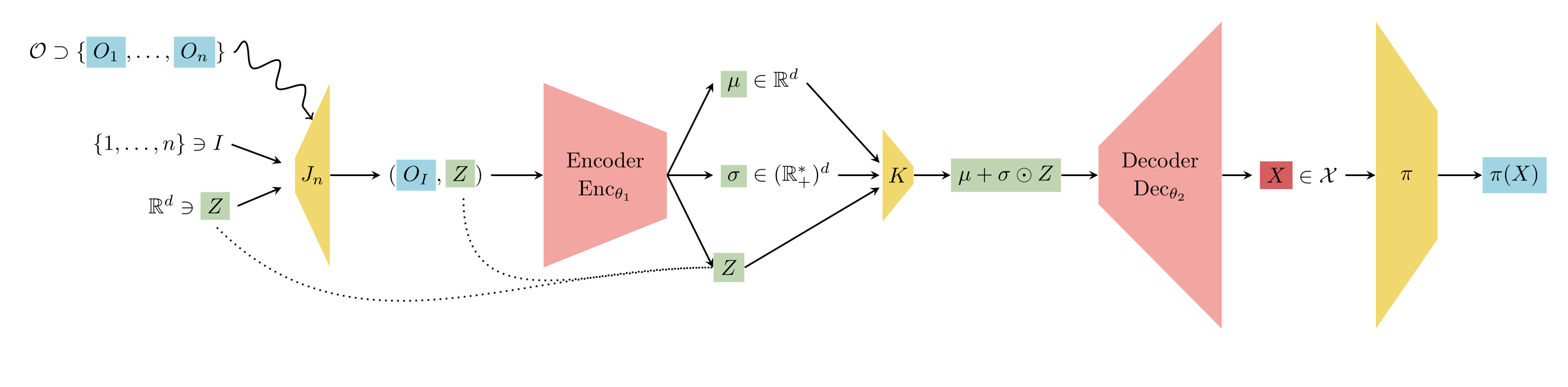
variables in $\calO$. @fig-VAE illustrates the architecture of the VAE used
in this study. It shows the key components of the model, including the
encoder, the latent space, and the decoder, along with the flow of information
between them.
:::{#fig-VAE}
{width=700}
Architecture of the simulator. The figure depicts the flow of information
through the encoder, latent space, and decoder components. It emphasizes how
the input source of randomness $Z$ is transformed into a latent representation
and then reconstructed as a complete data, $X=\Gen_{\theta}(Z)$, which can be
mapped to a real-world data $O=\pi(X)$.
:::
The word "auto-encoder" reflects the nature of the parametric form of each
$\Gen_{\theta}$. We begin with a formal presentation in four steps, which is
then followed by a discussion of what each step implements. Specifically,
each $\Gen_{\theta}$ writes as a composition of four mappings $J_{n}$,
$\Enc_{\theta_{1}}$, $K$ and $\Dec_{\theta_{2}}$ with $\theta := (\theta_{1},
\theta_{2}) \in \Theta_{1} \times \Theta_{2} = \Theta$:
$$
\Gen_{\theta} = \Dec_{\theta_{2}} \circ K \circ \Enc_{\theta_{1}} \circ
J_{n}.
$$
Here,
1. $J_{n}: \{1, \ldots, n\} \times \bbR^{d} \to \calO \times \bbR^{d}$ is
such that
$$
J_{n} (Z) = (O_{i}, (Z^{(1)}, \ldots, Z^{(d)}))
$$
with $i = Z^{(0)}$;
2. $\Enc_{\theta_{1}} : \calO \times \bbR^{d} \to \bbR^{d} \times
(\bbR_{+}^{*})^{d} \times \bbR^{d}$ is such that,
if $\Enc_{\theta_{1}}(o,z) = (\mu, \sigma, z')$, then
- $z=z'$, and
- $\Enc_{\theta_{1}}(o,z'') = (\mu, \sigma, z'')$ for all $z''\in\bbR^{d}$;
3. $K : \bbR^{d} \times (\bbR_{+}^{*})^{d} \times \bbR^{d} \to \bbR^{d}$ is
given by
$$
K(\mu,\sigma,z) := \mu + \sigma \odot z,
$$
where $\odot$ denotes the componentwise product;
4. $\Dec_{\theta_{2}}$ maps $\bbR^{d}$ to $\calX$.
Conditionally on $O^{1:n}$ and $Z$, the computation of $\Gen_{\theta} (Z)$ is
deterministic. The process unfolds in four steps:
1. **Sampling and transfer.** Compute $J_{n}(Z)$, which involves sampling
one observation $O_{i}$ uniformly among all genuine observations and transfer
$(Z^{(1)}, \ldots, Z^{(d)})$ unchanged.
2. **Encoding step.** Compute $\Enc_{\theta_{1}} \circ J_{n}(Z)$, which
encodes $O_{i}$ as a vector $\mu \in \bbR^{d}$ and a $d\times d$ covariance
matrix $\diag(\sigma)^2$. This step does not modify $(Z^{(1)}, \ldots,
Z^{(d)})$, which is transferred unchanged.
3. **Gaussian sampling.** Compute $K\circ \Enc_{\theta_{1}} \circ J_{n}(Z)$ by
evaluating $\mu + \sigma \odot (Z^{(1)}, \ldots, Z^{(d)}) \in \bbR^{d}$. This
amounts to sampling from the Gaussian law with mean $\mu$ and covariance
matrix $\diag(\sigma)^2$. In other words, $K$ enables the sampling of a
neighbor of the encoded version of $O_i$ in the latent space.
4. **Decoding step.** Compute $\Dec_{\theta_{2}}\circ K\circ \Enc_{\theta_{1}}
\circ J_{n}(Z)$, which maps the encoded version of $O_{i}$, that is, $\mu +
\sigma \odot (Z^{(1)}, \ldots, Z^{(d)})$, to an element of $\calX$.
## Formal training
Formally, training the VAE involves maximizing the likelihood of $O^{1:n}$
within a parametric model of laws by maximizing a lower bound of the
likelihood. This process begins with the introduction of a working model of
mixtures for $P$. The working model (undoubtedly flawed) postulates the
existence of a latent random variable $U\in \bbR^{d}$ and a parametric model
of *tractable* conditional densities
$$
\{o \mapsto p_{\theta_{2}} (o|u) : u \in \bbR^{d},
\theta_{2} \in \Theta_{2}\}
$$
such that
- $U$ is drawn from the standard Gaussian law on $\bbR^{d}$;
- there exists $\theta_{2} \in \Theta_{2}$ such that, given $U$, $O$ is drawn
from $p_{\theta_{2}} (\cdot|U)$.
Here, tractable densities refer to those that can be easily worked with
analytically, while in contrast, intractable densities are too complex to
handle directly.
Therefore, the working model (undoubtedly flawed) postulates the existence of
$\theta_{2} \in \Theta_{2}$ such that $P$ admits the generally *intractable*
density
$$
o \mapsto \int p_{\theta_{2}}(o|u) \phi_{d}(u)du
$$
where $\phi_{d}$ denotes the density of the standard Gaussian law on
$\bbR^{d}$. As suggested by the use of the parameter $\theta_{2}$, the
definition of the conditional densities $p_{\theta_{2}}(\cdot|u)$ ($u \in
\bbR^{d}$) involves the decoder $\Dec_{\theta_{2}}$.
Since directly maximizing the likelihood of $O^{1:n}$ under the working model
is infeasible, a *secondary* parametric model of *tractable* conditional
densities is introduced:
$$
\{u \mapsto g_{\theta_{1}} (u|O_{i}) : 1 \leq i \leq n, \theta_{1} \in
\Theta_{1}\}
$$
to model the conditional laws of $U$ given $O_{1}$, given $O_{2}$, $\ldots$,
given $O_{n}$. Here too, the use of the parameter $\theta_{1}$ indicates that
the definition of the conditional densities $g_{\theta_{1}} (\cdot|O_{i})$ ($1
\leq i \leq n$) involves the encoder $\Enc_{\theta{1}}$.
Now, by Jensen's inequality, for any $1 \leq i \leq n$ and all
$\theta = (\theta_{1}, \theta_{2})\in \Theta$,
$$
\begin{aligned}
\log p_{\theta_{2}}(O_{i})
&= \log \int p_{\theta_{2}} (O_{i}|u)
\frac{\phi_{d}(u)}{g_{\theta_{1}}(u|O_{i})} g_{\theta_{1}}(u|O_{i}) du\\
&\geq \int \log\left(p_{\theta_{2}} (O_{i}|u)
\frac{\phi_{d}(u)}{g_{\theta_{1}}(u|O_{i})}\right) g_{\theta_{1}}(u|O_{i})
du\\
&= -\KL(g_{\theta_{1}}(\cdot|O_{i}); \phi_{d}) +
E_{U\sim g_{\theta_{1}}(\cdot|O_{i})} [\log p_{\theta_{2}}(O_{i}|U)]=:
\LB_{\theta}(O_{i}),
\end{aligned}
$${#eq-LB}
where $\KL$ denotes the Kullback-Leibler divergence and $U$ in the expectation
is drawn from the conditional law with density $g_{\theta_{1}}(\cdot |
O_{i})$. The notation $\LB$ is used to indicate that it represents a lower
bound. Thus, the likelihood of $O^{1:n}$ under $\theta_{2} \in \Theta_{2}$ is
lower-bounded by
$$
\sum_{i=1}^{n} \LB_{\theta}(O_{i})
$$
for all $\theta_{1} \in \Theta_{1}$. As suggested earlier, training the VAE
formally consists of solving
$$
\max_{\theta\in\Theta} \left\{\sum_{i=1}^{n}\LB_{\theta}(O_{i})\right\}
$${#eq-VAE}
rather than solving
$$
\max_{\theta_{2} \in \Theta_{2}} \left\{\sum_{i=1}^{n} \log p_{\theta_{2}}
(O_{i})\right\}.
$$
# How to build the VAE {#sec-build-VAE}
## A formal description {#sec-VAE-formal}
We implement the classes of encoders and decoders, that is
$\{\Enc_{\theta_{1}} : \theta_{1} \in \Theta_{1}\}$ and $\{\Dec_{\theta_{2}} :
\theta_{2} \in \Theta_{2}\}$, as neural network models. Each encoder
$\Enc_{\theta_{1}}$ and decoder $\Dec_{\theta_{2}}$ consist of a stack of
layers of two types: *densely-connected* and *activation* layers (linear, $x
\mapsto x$; ReLU : $x \mapsto \max(0, x)$, softmax: $(x_{1}, x_{2}) \mapsto
(e^{x_{1}}, e^{x_{2}})/(e^{x_{1}} + e^{x_{2}})$). The neural networks are
rather simple in design, but nevertheless (moderately) high-dimensional and
arguably over-parametrized, as discussed in @sec-over-parametrization.
The model $\{u \mapsto g_{\theta_{1}}(u|O_{i}) : 1 \leq i \leq n, \theta_{1}
\in \Theta_{1}\}$ is chosen such that $U$ drawn from
$g_{\theta_{1}}(\cdot|O_{i})$ is a Gaussian vector with mean $\mu_{i}$ and
covariance matrix $\diag(\sigma_{i})^{2}$ where $\Enc_{\theta_{1}}(O_{i},
\cdot) = (\mu_{i}, \sigma_{i}, \cdot)$, that is, when the
$\theta_{1}$-specific encoding of $O_{i}$ equals $(\mu_{i}, \sigma_{i})$.
Remarkably, the left-hand side term in the definition of $\LB_{\theta}(O_{i})$
(@eq-LB) is then known in closed form:
$$
-\KL(g_{\theta_{1}}(\cdot|O_{i}); \phi_{d}) = \tfrac{1}{2} \sum_{j=1}^{d}
\left(1 + \log (\sigma_{i}^{2})_{j} - (\sigma_{i}^{2})_{j} - (\mu_{i}^{2})_{j}
\right),
$${#eq-LB-LHS-term}
where $(\mu_{i}^{2})_{j}$ and $(\sigma_{i}^{2})_{j}$ are the $j$-th components
of $\mu_{i} \odot \mu_{i}$ and $\sigma_{i} \odot \sigma_{i}$, respectively.
This is very convenient, because @eq-LB-LHS-term makes estimating the term
$\KL(g_{\theta_{1}}(\cdot|O_{i}); \phi_{d})$ unnecessary, a task that would
otherwise introduce more variability in the procedure.
As for the model $\{o \mapsto p_{\theta_{2}}(o|u) : u \in \bbR^{d}, \theta_{2}
\in \Theta_{2}\}$, the only requirement is that it must be chosen in such a
way that $\log p_{\theta_{2}}(O_{i} | u)$ be computable for all $1\leq i \leq
n$, $\theta_{2} \in \Theta_{2}$ and $u \in \bbR^{d}$. This is not a tall
order as soon as $O$ can be decomposed as a sequence of (e.g., time-ordered)
random variables that are vectors with categorical, or integer or real
entries. Indeed, it then suffices (i) to decompose the likelihood accordingly
under the form of a product of conditional likelihoods, and (ii) to choose a
tractable parametric model for each factor in the decomposition. We
illustrate the construction of $\{o \mapsto p_{\theta_{2}}(o|u) : u \in
\bbR^{d}, \theta_{2} \in \Theta_{2}\}$ in the context of our running example.
::: {.callout-note appearance="simple"}
## Running example, cted.
In the context of this example, $O=(V,W,A,Y)$ with $V \in \{0,1\}^{2}$, $W \in
\bbR^{3}$, $A\in\{0,1\}$ and $Y\in\bbR$. Since the source of randomness $Z$
has dimension $(d+1)$, $d$ must satisfy $d = d_{1} + 3$ for some integer
$d_{1} \geq 1$.
Set $\theta = (\theta_{1}, \theta_{2})\in \Theta$, $u \in \bbR^{d}$, and let
$\pi\circ \Dec_{\theta_{2}} (u) = (\tilde{v}, \tilde{w}, \tilde{a}, \tilde{y})
\in \calO$. The conditional likelihood $p_{\theta_{2}}(O|u)$ (of $O$ given
$U=u$) equals
$$
p_{\theta_{2}}(V,W|u) \times p_{\theta_{2}}(A|W,V,u) \times p_{\theta_{2}}(Y|A,W,V,u)
$$
so it suffices to define the conditional likelihoods $p_{\theta_{2}}(V,W|u)$
(of $(V,W)$ given $U=u$), $p_{\theta_{2}}(A|W,V,u)$ (of $A$ given $(W,V)$ and
$U=u$) and $p_{\theta_{2}}(Y|A,W,V,u)$ (of $Y$ given
$(A,W,V)$ and $U=u$).
- We decide that $V$ and $W$ are conditionally independent given $U$ under
$p_{\theta_{2}}(\cdot|u)$. Therefore, it suffices to characterize the
conditional likelihoods $p_{\theta_{2}}(V|u)$ (of $V$ given $U=u$) and
$p_{\theta_{2}}(W|u)$ (of $W$ given $U=u$).
- We choose $w\mapsto p_{\theta_{2}}(w|u)$ to be the Gaussian density with
mean $\tilde{w}$ and identity covariance matrix.
:::
::: {.callout-note appearance="simple"}
## Running example, cted.
- The description of the conditional law of $V$ given $U=u$ under
$p_{\theta_{2}}(\cdot|u)$ is slightly more involved. It requires that we give
more details on the encoders and decoders.
- Like every encoder, $\Enc_{\theta_{1}}$ actually maps $\calO \times
\bbR^{d}$ to $[\bbR^{d_{1}}\times \{0\}^{3}] \times
[(\bbR_{+}^{*})^{d_{1}} \times \{1\}^{3}] \times \bbR^{d}$. In words, if
$\Enc_{\theta_{1}}(o, \cdot) = (\mu, \sigma, \cdot)$, then it necessarily
holds that the three last components of $\mu$ and $\sigma$ are 0 and 1,
respectively. Therefore the three last components of the random vector $K
\circ \Enc_{\theta_{1}} \circ J_{n}(Z)$ equal $Z^{(d-2)}, Z^{(d-1)},
Z^{(d)}$, three independent standard normal random variables.
- To compute $\Dec_{\theta_{2}}(u) = (\tilde{v}, \tilde{w}, \tilde{y}_{0},
\tilde{y}_{1}, \tilde{a}) \in \calX$, we actually compute $\tilde{w}$
*then* $\tilde{v}$, *then* $(\tilde{y}_{0}, \tilde{y}_{1},\tilde{a})$.
- The output $\tilde{w}$ is a $\theta_{2}$-specific deterministic
function of the first $d_{1}$ components of $u$.
- The output $\tilde{v}$ is a $\theta_{2}$-specific deterministic
function of the $(d_{1}+2)$ first components of $u$.
More specifically, two (latent) probabilities $\tilde{g}_{1},
\tilde{g}_{2}$ are first computed, as $\theta_{2}$-specific
deterministic functions of the $d_{1}$ first components of $u$. Then
$\tilde{v}_{1}$ and $\tilde{v}_{2}$ are set to
$\textbf{1}\{\Phi(u^{(d_{1}+1)}) \leq \tilde{g}_{1}\}$ and
$\textbf{1}\{\Phi(u^{(d_{1}+2)}) \leq \tilde{g}_{2}\}$, where $\Phi$
denotes the standard normal cumulative distribution function (c.d.f)
and $u^{(d_{1}+1)}, u^{(d_{1}+2)}$ are the $(d_{1}+1)$-th and
$(d_{1}+2)$-th components of $u$.
For instance, $\tilde{v}_{1}$ is given the value 1 if
$\Phi(u^{(d_{1}+1)}) \leq \tilde{g}_{1}$ and 0 otherwise. Note that
$\textbf{1}\{\Phi(Z^{(d_{1}+1)}) \leq \tilde{g}_{1}\}$ follows the
Bernoulli law with parameter $\tilde{g}_{1}$ because $Z^{(d_{1}+1)}$
is drawn from the standard normal law.
- The output $(\tilde{y}_{0},
\tilde{y}_{1})$ is a $\theta_{2}$-specific deterministic function of
$(\tilde{v}, \tilde{w})$ and the $d_{1}$ first components of $u$.
- The output $\tilde{a}$ is a $\theta_{2}$-specific deterministic
function of $(\tilde{v}, \tilde{w})$ and the last component of $u$.
More specifically, a (latent) probability $\tilde{h}$ is first
computed, as a $\theta_{2}$-specific deterministic function of
$(\tilde{v}, \tilde{w})$. Then $\tilde{a}$ is set to
$\textbf{1}\{\Phi(u^{(d)}) \leq \tilde{h}\}$.
Note that $\textbf{1}\{\Phi(Z^{(d)}) \leq \tilde{h}\}$ follows the
Bernoulli law with parameter $\tilde{h}$ because $Z^{(d)}$ is drawn
from the standard normal law.
We are now in a position to describe the conditional law of $V$ given
$U=u$. We decide that, conditionally on $U=u$, under
$p_{\theta_{2}}(\cdot|u)$, $V_{1}$ and $V_{2}$ are independently drawn
from the Bernoulli laws with parameters $\tilde{g}_{1}$ and
$\tilde{g}_{2}$. Thus, $p_{\theta_{2}}(\cdot|u)$ is such that
$p_{\theta_{2}}(v|u) = [v_{1} \tilde{g}_{1} + (1-v_{1})(1-\tilde{g}_{1})]
\times [v_{2} \tilde{g}_{2} + (1-v_{2})(1-\tilde{g}_{2})]$ for $v=(v_{1},
v_{2}) \in \{0,1\}^{2}$.
:::
::: {.callout-note appearance="simple"}
## Running example, cted.
- The description of the conditional law of $A$ given $(W, V)$ and $U=u$ under
$p_{\theta_{2}}(\cdot|u)$ is similar to that of $V$ given $U$. We decide
that, conditionally on $(W, V)$ and $U=u$, under $p_{\theta_{2}}(\cdot|W, V,
u)$, $A$ follows the Bernoulli law with parameter
$\tilde{\underline{h}}(V,W)$, where the probability
$\tilde{\underline{h}}(v,w)$ lies between $\tilde{h}$ and
$\bar{A}_{n}:=\tfrac{1}{n}\sum_{i=1}^{n} A_{i}$ and is given, for any $(v,w)
\in \{0,1\}^{2} \times \bbR^{3}$, by
$$
\begin{aligned}
\tilde{\underline{h}}(v,w) :=& t(v,w) \tilde{h} + [1 - t(v,w)] \bar{A}_{n} \quad \text{with}\\
-10\log t(v,w) =& - \left[v_{1} \log \tilde{g}_{1} + (1-v_{1}) \log
(1-\tilde{g}_{1})\right]\\
& - \left[v_{2} \log \tilde{g}_{2} + (1-v_{2}) \log (1-\tilde{g}_{2})\right]\\
&+\|w - \tilde{w}\|_{2}^{2}.
\end{aligned}
$$
Thus, $p_{\theta_{2}}(\cdot|W,V,u)$ is such that $p_{\theta_{2}}(a|W,V,u)
= a \tilde{\underline{h}(V,W)} + (1-a)(1-\tilde{\underline{h}}(V,W))$ for
$a \in \{0,1\}$.
- Finally, we choose $y \mapsto p_{\theta_{2}}(y|A,W,V,u)$ to be the
two-regime density given by
$$
p_{\theta_{2}}(y|A,W,V,u) =
\frac{\textbf{1}\{A=\tilde{a}\}}{\tilde{s}(W)} \phi_{1}
\left(\frac{y - \tilde{y}}{\tilde{s}(W)}\right) + \textbf{1}\{A\neq
\tilde{a}\} C^{-1}
$$
where $\tilde{s}(w):= \tfrac{1}{\sqrt{5}} \|w - \tilde{w}\|_{2}$ for any $w \in
\bbR^{3}$ and $C$ is the
Lebesgue measure of the support of the marginal law of $Y$ under $P$ (it
does not matter if $C$ is unknown).
Thus, two cases arise:
- If $A = \tilde{a}$, then $Y$ is conditionally drawn under
$p_{\theta_{2}}(\cdot|A,W,V,u)$ from the Gaussian law with mean $\tilde{y} =
a \tilde{y}_{1} + (1-a) \tilde{y}_{0}$
and variance $\tilde{s}(W)^{2}$.
- Otherwise, $Y$ is conditionally drawn under
$p_{\theta_{2}}(\cdot|A,W,V,u)$ from the uniform law on the support of the
marginal law of $Y$ under $P$.
Therefore, the conditional likelihood $p_{\theta_{2}}(Y|A,W,V,u)$ bears
information only if $A=\tilde{a}$ (that is, if the actions $A$ and
$\tilde{a}$ undertaken when generating $O=(V,W,A,Y)$ and computing
$\Dec_{\theta_{2}}(u)$ coincide), which can be interpreted as a necessary
condition to justify the comparison of the rewards $Y$ and
$\tilde{y}$. Moreover, when $A=\tilde{a}$, the closer are the contexts $W$
and $\tilde{w}$, the more relevant is the comparison and the larger the
magnitude of $p_{\theta_{2}}(Y|A,W,V,u)$ can be.
:::
::: {.callout-note appearance="simple"}
## Running example, cted.
In summary, the right-hand side term in the definition of
$\LB_{\theta}(O_{i})$ @eq-LB equals, up to a term that does not depend on
$\theta$,
$$ \begin{aligned}
\tfrac{1}{2}E_{U \sim g_{\theta_{1}}(\cdot|O_{i})} \Bigg[
& -2\left(V_{1,i} \log \tilde{G}_{1} + (1-V_{1,i}) \log (1 -
\tilde{G}_{1})\right) \\
& -2\left(V_{2,i} \log \tilde{G}_{2} + (1-V_{2,i}) \log (1 -
\tilde{G}_{2})\right) \\
& - \|W_{i} - \tilde{W}\|_{2}^{2}\\
& -2\left(A_{i} \log \tilde{\underline{H}} + (1-A_{i}) \log [1 -
\tilde{\underline{H}}]\right)\\
& -\textbf{1}\{A_{i} = \tilde{A}\} \times \left(\log \tilde{S}(W_{i})^{2} +
\frac{(Y_{i} - \tilde{Y})^{2}}{2\tilde{S}(W_{i})^{2}}\right)\Bigg],
\end{aligned}
$${#eq-log-p-theta2}
with the notational conventions $\pi \circ \Dec_{\theta_{2}} (U) = (\tilde{V},
\tilde{W}, \tilde{A}, \tilde{Y})$, $V_{i} = (V_{i,1}, V_{i,2})$, and where
$\tilde{G}_{1}$, $\tilde{G}_{2}, \tilde{\underline{H}}, \tilde{S}$
are defined like the
above latent quantities $\tilde{g}_{1}$, $\tilde{g}_{2}, \tilde{\underline{h}},
\tilde{s}$
with $U$ substituted for $u$. The expression is easily interpreted: the
opposite of @eq-log-p-theta2 is an average risk that measures
- the likelihood of $V_{i,1}$ and $V_{i,2}$ from the points of view of the
Bernoulli laws with parameters $\tilde{G}_{1}$ and $\tilde{G}_{2}$ (first and
second terms),
- the average proximity between $W_{i}$ and $\tilde{W}$ (third term),
- the likelihood of $A_{i}$ from the point of view of the Bernoulli law with
parameter $\tilde{\underline{H}}$ (fourth term),
- the average proximity between $Y_{i}$ and $\tilde{Y}$ (fifth term) *only if*
$A_{i} = \tilde{A}$ (otherwise, the comparison would be meaningless).
In other terms, the opposite of @eq-log-p-theta2 can be interpreted as a
measure of the average faithfulness of the reconstruction of $O_{i}$ under the
form $\pi \circ \Dec_{\theta_{2}} (U)$ with $U$ drawn from
$g_{\theta_{1}}(\cdot|O_{i})$. The larger is @eq-log-p-theta2, the better is
the reconstruction of $O_{i}$ under the form $\pi \circ \Dec_{\theta_{2}} (U)$
with $U$ drawn from $g_{\theta_{1}}(\cdot|O_{i})$.
To conclude, note that the conditional laws of $W$ and $Y$, both Gaussian,
could easily be associated with diagonal covariance matrices different from
the identity matrix. This adjustment would be particularly relevant in
situations where $\|W\|_{2}$ and $|Y|$ are typically not of the same
magnitude, with $O=(V,W,A,Y)$ drawn from the law $P$ of the experiment of
interest. Alternatively, the genuine observations could be pre-processed to
ensure that $\|W\|_{2}$ and $|Y|$ are brought to comparable magnitudes.
:::
The hope is that, once the VAE is trained, yielding a parameter $\thn =
((\thn)_{1}, (\thn)_{2})$, the corresponding generator $\Gen_{\thn}$ produces
a synthetic complete data $X\in\calX$ such that the law of $\pi(X) \in\calO$
closely approximates $P$. Naturally, this approximation is closely related to
the conditional densities $g_{(\thn)_{1}}(\cdot|O_{i})$ and
$p_{(\thn)_{2}}(\cdot | u)$ ($1 \leq i \leq n$, $u \in \bbR$).
For instance, in the context of the running example, if $O = (V,W, A, Y) = \pi
\circ \Gen_{\thn}(Z)$ and if $\xi, \zeta$ are independently drawn from the
centered Gaussian laws with an identity covariance matrix on $\bbR^{3}$ and
variance 1 on $\bbR$, respectively, then $(W + \xi, A, Y + \zeta)$ follows a
law that admits the density
$$
\begin{aligned}
(v, w, a, y)\mapsto \int & p_{(\thn)_{2}}(y|a, w, v, u) \times
\textbf{1}\{a=\tilde{a}_{(\thn)_{2}}(u)\}\\
& \times
p_{(\thn)_{2}}(w,v|u)\left(\frac{1}{n}\sum_{i=1}^{n}
g_{(\thn)_{1}}(u |O_{i}) \right) du,
\end{aligned}
$$
where $\tilde{a}_{(\thn)_{2}}(u)$ is defined as the $A$-coefficient of
$\pi\circ \Dec_{(\thn)_{2}}(u)$.
## About the over-parametrization {#sec-over-parametrization}
In @sec-VAE-formal we acknowledged that the models $\{\Enc_{\theta_{1}} :
\theta_{1} \in \Theta_{1}\}$ and $\{\Dec_{\theta_{2}} : \theta_{2} \in
\Theta_{2}\}$ are over-parametrized in the sense that the dimensions of the
parameter set $\Theta_{1}\times \Theta_{2}$ is potentially large. For
instance, the dimension of the model that we build in the next section is
1157. This is a common feature of neural networks.
Our models are also over-parametrized in the sense that they are not
identifiable. This is obviously the case because of the loss of information
that governs the derivation of an observation $O$ as a piece $\pi(X)$ of a
complete data $X$ that we are not given to observe in its entirety.
::: {.callout-note appearance="simple"}
## Running example, cted.
In particular, in the context of this example, it is well know that we cannot
learn from $O_{1}, \ldots, O_{n}$ any feature of the joint law of the
counterfactual random variables $(Y[0], Y[1])$ that does not reduce to a
feature of the marginal laws of $Y[0]$ or $Y[1]$, unless we make very strong
assumptions on this joint law (e.g., that $Y[0]$ and $Y[1]$ are independent).
:::
This is not a source of concern. First, it is generally recognized that the
fitting of neural networks often benefits from the high dimensionality of the
optimization space and the presence of numerous equivalently good local
optima, resulting in a redundant optimization landscape
[@choromanska2015loss], [@arora2018optimization]. Second, our objective is to
construct a generator that approximates the law $P$ of $O_{1}, \ldots, O_{n}$,
generating $O\in\calO$ by first producing $X\in\calX$ (via $\Gen_{\theta}(Z)$)
and then providing $\pi(X)$. The fact that two different generators
$\Gen_{\theta}$ and $\Gen_{\theta'}$ can perform equally well is not
problematic. Identifying *one* generator $\Gen_{\theta}$ that performs well
is sufficient.
It is possible to search for generators that satisfy user-supplied
constraints, provided these can be expressed as a real-valued criterion
$F(E[\calC(\Gen_{\theta}(Z))])$. For example, one may wish to construct a
generator $\Gen_{\theta}$ such that the components of $X$ under
$\law(\Gen_{\theta})$ exhibit a pre-specified correlation pattern (as
demonstrated in the simple example below).
To focus the optimization procedure on generators that approximately meet
these constraints, one can modify the original criterion @eq-VAE by adding a
penalty term. Specifically, given a user-supplied hyper-parameter $\lambda >
0$, we can substitute
$$
\max_{\theta\in\Theta} \left\{\sum_{i=1}^{n}\LB_{\theta}(O_{i}) +
\lambda F(E_{Z \sim \Unif\{1, \ldots, n\} \otimes N(0,1)^{\otimes
d}}[\calC(\Gen_{\theta}(Z))])\right\}
$${#eq-penalized-VAE}
for @eq-VAE. From a computational perspective, this adjustment simply
involves adding the term
$$
\lambda F\left(\frac{1}{m}\sum_{i=1}^{m} \calC(\Gen_{\theta} (Z_{m+i}))\right)
$${#eq-penalization-VAE}
to the expressions within the curly brackets in the definition of $g$ in the
algorithm described in @sec-algo.
::: {.callout-note appearance="simple"}
## Running example, cted.
In particular, in the context of this example, we could look for generators
$\Gen_{\theta}$ such that the correlation of $Y[0]$ and $Y[1]$ under
$\law(\Gen_{\theta} (Z))$ be close to a target correlation $r \in ]-1, 1[$.
In that case, we could choose $\calC(\Gen_{\theta} (Z)) := (Y[0]Y[1],
Y[0]^{2}, Y[1]^{2}, Y[0], Y[1])$ and $F : (a,b,c,d,e) \mapsto |(a -
de)/\sqrt{(b - d^2)(c - e^2)} - r|$.
:::
# Implementation of the VAE in the context of the running example {#sec-implementation-VAE}
We now show how to implement the classes of encoders and decoders, hence of
generators, in the context of our running example. We will also define other
loss functions that are needed to train the model.
We implemented our approach using the
[TensorFlow](https://www.tensorflow.org/) package, but also experimented with
[PyTorch](https://pytorch.org/). Both frameworks yielded similar results,
with no noticeable differences in performance. However, we found TensorFlow
to be slightly more beginner-friendly, which might make it easier for readers
new to neural network frameworks to follow our implementation.
## Implementing the encoder
The first chunk of code defines a function, namely `build_encoder`, to build
$\Enc_{\theta_{1}}$. The parameter `latent_dim` is the `Python` counterpart
of $d_{1}$. The parameters `nlayers_encoder` and `nneurons_encoder` are the
numbers of layers and of neurons in each layer, respectively. The parameter
`L` will be discussed later.
```{python building-encoder}
#| message: false
#| warning: false
import os
os.environ['TF_CPP_MIN_LOG_LEVEL'] = '2'
import tensorflow as tf
from tensorflow.keras import Input, Model
from tensorflow.keras.layers import Lambda, Dense, Activation, concatenate,\
  Reshape, Concatenate
import tensorflow.keras.backend as KK
## import tensorflow_probability as tfp

def build_encoder(dimW,
                  dimV,
                  latent_dim,
                  L,
                  nlayers_encoder,
                  nneurons_encoder):
  if isinstance(nneurons_encoder, int):
    nneurons_encoder = np.array([nneurons_encoder])
  if not (nlayers_encoder is None):
    if len(nneurons_encoder) == 1:
      nneurons_encoder = np.repeat(nneurons_encoder, nlayers_encoder)
    elif not (len(nneurons_encoder) == nlayers_encoder):
      print("Inconsistency of 'nneurons' and 'nlayers' in the encoder's definition...\n")
  dimWV = dimW + dimV
  nlayers_encoder = len(nneurons_encoder)
  e_obs_input = Input(shape = (dimWV + 2,),
                      name = "e_obs_input")
  e_alea_input = Input(shape = (L, latent_dim + dimV + 1, ),
                        name = "e_alea_input")
  e = Dense(nneurons_encoder[0],
            name = "dense_e_" + str(0),
            activation = "relu")(e_obs_input)
  for i in range(nlayers_encoder - 2):
    e = Dense(nneurons_encoder[i + 1],
              name = "dense_e_" + str(i + 1),
              activation = "relu")(e)
  mu = Dense(latent_dim,
              name = "mu")(e)
  zeros = KK.zeros_like(mu)
  zeros = Lambda(lambda x: x[:, :(dimV + 1)], name="zeros")(zeros)
  mu = Concatenate(axis = 1,
                   name = "concatenate_mu_zeros")([mu, zeros])
  log_sigma = Dense(latent_dim,
                    name = "log_sigma")(e)
  log_sigma = Lambda(lambda x: -tf.math.exp(x), name = "minus_exponential")(log_sigma)
  log_sigma = Concatenate(axis = 1,
                          name = "concatenate_log_sigma_zeros")([log_sigma, zeros])
  param = Concatenate(name = "param")([mu, log_sigma])
  encoder = Model(inputs = [e_obs_input, e_alea_input],
                  outputs = [param, e_alea_input])
  return encoder
```
The code related to encoding is complete.
## Implementing the decoder
The first chunk of code defines the component of $\Dec_{\theta_{2}}$, namely
`build_WV_decoder`, that generates $(V,W)$ based on $U$. It also defines a
function, `as_sample`, that allows to *approximately* draw from a discrete
distribution. The parameters `nlayers_WV_decoder` and `nneurons_WV_decoder`
are the numbers of layers and of neurons in each layer, respectively. The
parameter `L` will be discussed later.
We say that `as_sample` allows to sample *approximately* from a discrete
distribution since we cannot simply draw from it
because of the need for this operation to be differentiable with respect to
(w.r.t.) the parameters of the neural network. Instead, we use the fact that,
for $\beta>0$ a large constant and $Z$ a standard normal random variable, the
law of the random variable
$$
\expit(-\beta(\Phi(Z) - p))
$${#eq-approximately-bernoulli}
(recall that $\Phi$ is the c.d.f. of the standard
normal law) is concentrated around $\{0,1\}$, a small neighborhood of $1$ having mass
approximately $p$ and a small neighborhood of $0$ having mass approximately
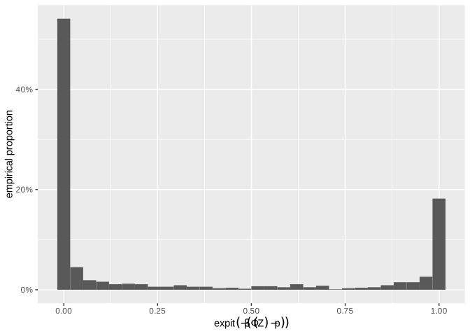
$(1-p)$. For instance @fig-approximately-bernoulli shows the empirical
cumulative distribution function of 1000 independent copies of the random
variable defined in @eq-approximately-bernoulli with $\beta=30$ and $p=1/3$:
```{r}
#| label: fig-approximately-bernoulli
#| fig-cap: Empirical c.d.f. of 1000 independent copies of the random variable defined in @eq-approximately-bernoulli with $\beta=30$ and $p=1/3$. The law is close the Bernoulli law with parameter $\tfrac{1}{3}$.
#| message: false
library(magrittr)
beta <- 30
p <- 1/3
tibble::tibble(Z = stats::rnorm(1e3)) %>%
  dplyr::mutate(U = stats::pnorm(Z)) %>%
  dplyr::mutate(V = stats::plogis(-beta * (U - p))) %>%
  ggplot2::ggplot() +
  ggplot2::geom_histogram(ggplot2::aes(x = V,
                                       y = ggplot2::after_stat(count/sum(count)))) +
  ggplot2::scale_y_continuous(labels = scales::percent) +
  ggplot2::xlab(quote(expit(-beta(Phi(Z) - p)))) +
  ggplot2::ylab("empirical proportion")
```
```{python VW-decoder}
import sys

def as_sample(tensors, beta = 30):
  probs = tensors[0] # (pi_v)_{v in {0,...,nb_cat - 1}} where pi_v = P(V = v)
  nb_cat = probs.shape[2]
  Z = tensors[1] # the source of randomness
  U = tfp.distributions.Normal(loc = 0, scale = 1).cdf(Z)
  Pi = KK.cumsum(probs, axis = 2) # computing (Pi_v)_{v in {0,...,nb_cat - 1}}
  Pi_prev = Pi[..., 0]
  as_V = KK.sigmoid(-beta * (U - Pi_prev)) # Z[0] ~= 1_{U<pi_0}
  as_V = tf.expand_dims(as_V, -1)
  for v in range(nb_cat - 2):
    Pi_next = Pi[..., v + 1]
    as_V_v = KK.sigmoid(- beta * (U - Pi_next)) - KK.sigmoid(- beta * (U - Pi_prev))
    as_V_v = tf.expand_dims(as_V_v, -1)
    Pi_prev = Pi_next
    as_V = concatenate([as_V, as_V_v])
  Pi_last = Pi[..., nb_cat - 2]
  as_V_v = 1 - KK.sigmoid(- beta * (U - Pi_last))
  as_V_v = tf.expand_dims(as_V_v, -1)
  as_V = concatenate([as_V, as_V_v])
  return as_V

def build_WV_decoder(dimW,
                     dimV,
                     nb_cat_V,
                     latent_dim,
                     L,
                     nlayers_WV_decoder,
                     nneurons_WV_decoder,
                     activation_W = "linear"):
  if isinstance(nneurons_WV_decoder, int):
    nneurons_WV_decoder = np.array([nneurons_WV_decoder])
  if not (nlayers_WV_decoder is None):
    if len(nneurons_WV_decoder) == 1:
      nneurons_WV_decoder = np.repeat(nneurons_WV_decoder, nlayers_WV_decoder)
    elif not (len(nneurons_WV_decoder) == nlayers_WV_decoder):
      print("Inconsistency of 'nneurons' and 'nlayers' in the WV decoder's definition...\n")
  nlayers_WV_decoder = len(nneurons_WV_decoder)
  random_latent_vectors = Input(shape = (L, latent_dim + dimV, ),
                                name = "input_WV")
  alea = tf.slice(random_latent_vectors, (0, 0, latent_dim), (-1, -1, dimV))
  WV = tf.slice(random_latent_vectors, (0, 0, 0), (-1, -1, latent_dim))
  WV = Dense(nneurons_WV_decoder[0],
             name = "dense_WV_" + str(0),
             activation = "relu")(WV)
  for i in range(nlayers_WV_decoder - 1):
    WV = Dense(nneurons_WV_decoder[i + 1],
               name = "dense_WV_" + str(i + 1),
               activation = "relu")(WV)
  WV = Dense(dimW + dimV,
             name = "dense_WV_final")(WV)
  if dimW > 0:
    W = tf.slice(WV, (0, 0, 0), (-1, -1, dimW))
    W = Activation(activation_W,
                   name = "activation_W")(W)
  if dimV > 0:
    V_slice = tf.slice(WV, (0, 0, dimW), (-1, -1, 1))
    V_law = Dense(nb_cat_V[0],
                  activation = "softmax",
                  name = "softmax_V_0")(V_slice)
    V_random_latent_vectors = Lambda(lambda x: x[..., 0],
                                     name = "extr_V_alea_0")(alea)
    V = Lambda(as_sample,
               name = "as_V_0")([V_law, V_random_latent_vectors])
    V = Lambda(lambda x, y: tf.linalg.matmul(x, np.reshape(np.arange(y), (y, 1))),
               arguments={'y': nb_cat_V[0]},
               name = "lambda_V_0")(V)
    V = KK.cast(V, dtype = "float32")
    if dimV > 1:
      for v in range(dimV - 1):
        V_slice_v = tf.slice(WV, (0, 0, dimW + v + 1), (-1, -1, 1))
        V_law_v = Dense(nb_cat_V[v + 1],
                        activation = "softmax",
                        name = "softmax_V_" + str(v + 1))(V_slice_v)
        V_random_latent_vectors = Lambda(lambda x: x[..., v + 1],
                                         name = "extr_V_alea_" + str(v + 1))(alea)
        V_v = Lambda(as_sample,
                     name = "as_V_" + str(v + 1))([V_law_v, V_random_latent_vectors])
        V_v = Lambda(lambda x,y: tf.linalg.matmul(x, np.reshape(np.arange(y), (y, 1))),
                     arguments={'y': nb_cat_V[v+1]},
                     name = "lambda_V_" + str(v + 1))(V_v)
        V_v = KK.cast(V_v, dtype = "float32")
        V_law = concatenate([V_law, V_law_v])
        V = concatenate([V, V_v])

  if dimW > 0 and dimV > 0:
    WV = concatenate([W, V])
  elif dimW == 0:
    WV = V
  elif dimV == 0:
    WV = W
  else:
    sys.exit("One at least of 'dimW' and 'dimV' must be positive...\n")
  if dimV > 0:
    WV_decoder = Model(inputs = random_latent_vectors,
                       outputs = [WV, V_law],
                       name = "WV_decoder")
  else:
     WV_decoder = Model(inputs = random_latent_vectors,
                        outputs = WV,
                        name = "WV_decoder")
  return WV_decoder
```
The second chunk of code defines the component of $\Dec_{\theta_{2}}$, namely
`build_Alaw_decoder`, that generates a conditional law for $A$ given
$(V,W)$. The parameters `nlayers_Alaw_decoder` and `nneurons_Alaw_decoder` are
the numbers of layers and of neurons in each layer, respectively. The
parameter `L` will be discussed later.
```{python law-A-given-WV}
def build_Alaw_decoder(dimW,
                       dimV,
                       L,
                       nlayers_Alaw_decoder,
                       nneurons_Alaw_decoder):
  if isinstance(nneurons_Alaw_decoder, int):
    nneurons_Alaw_decoder = np.array([nneurons_Alaw_decoder])
  if not (nlayers_Alaw_decoder is None):
    if len(nneurons_Alaw_decoder) == 1:
      nneurons_Alaw_decoder = np.repeat(nneurons_Alaw_decoder, nlayers_Alaw_decoder)
    elif not (len(nneurons_Alaw_decoder) == nlayers_Alaw_decoder):
      print("Inconsistency of 'nneurons' and 'nlayers' in  the Alaw decoder's definition...\n")
  dimWV = dimW + dimV
  nlayers_Alaw_decoder = len(nneurons_Alaw_decoder)
  WV = Input(shape = (L, dimWV,), name = "input_Alaw")
  Alaw = Dense(nneurons_Alaw_decoder[0],
               name = "dense_Alaw_0",
               activation = "relu")(WV)
  if nlayers_Alaw_decoder > 1:
    for i in range(nlayers_Alaw_decoder-1):
      Alaw = Dense(nneurons_Alaw_decoder[i + 1],
                   name = "dense_Alaw_" + str(i + 1),
                   activation = "relu")(Alaw)
  Alaw = Dense(2,
               activation = "softmax",
               name = "dense_Alaw_final")(Alaw)
  Alaw_decoder = Model(inputs = WV,
                       outputs = Alaw,
                       name = "Alaw_decoder")
  return Alaw_decoder
```
The third chunk of code defines the component of $\Dec_{\theta_{2}}$, namely
`build_AYaY_decoder`, that generates the counterfactual outcomes $Y[0]$ and
$Y[1]$, the action carried out $A$ and the corresponding reward $Y$. The
parameters `nlayers_AYaY_decoder` and `nneurons_AYaY_decoder` are the numbers
of layers and of neurons in each layer, respectively. The parameter `L` will
be discussed later.
```{python Y0-Y1-A-Y-decoder}
def get_Y(tensors): # tensors[0]: (Y_{0}, Y_{1})
                    # tensors[1]: (1-A, A)
  Y = tensors[0] * tensors[1]
  Y = KK.sum(Y, axis = -1, keepdims = True)
  return Y

def trick_with_relu(x):
  out = tf.keras.activations.relu(x - 1/2)/(x - 1/2)
  out = tf.gather(out, 1, axis = 1)
  out = tf.expand_dims(out, -1)
  return out

def build_AYaY_decoder(dimW,
                       dimV,
                       latent_dim,
                       L,
                       nlayers_AYaY_decoder,
                       nneurons_AYaY_decoder,
                       activation_Ya = "linear"):
  if isinstance(nneurons_AYaY_decoder, int):
    nneurons_AYaY_decoder = np.array([nneurons_AYaY_decoder])
  if not (nlayers_AYaY_decoder is None):
    if len(nneurons_AYaY_decoder) == 1:
      nneurons_AYaY_decoder = np.repeat(nneurons_AYaY_decoder, nlayers_AYaY_decoder)
    elif not (len(nneurons_AYaY_decoder) == nlayers_AYaY_decoder):
      print("Inconsistency of 'nneurons' and 'nlayers' in the AYaY decoder's definition...\n")
  dimWV = dimW + dimV
  nlayers_AYaY_decoder = len(nneurons_AYaY_decoder)
  random_latent_vectors = Input(shape = (L, latent_dim + 1, ),
                                name = "alea_input_AYaY")
  WV = Input(shape = (L, dimWV, ),
             name = "WV_input_AYaY")
  Alaw = Input(shape = (L, 2,),
               name = "Alaw_input_AYaY")
  Arandom_latent_vectors = Lambda(lambda x: x[..., latent_dim],
                                  name = "extr_alea_AYaY")(random_latent_vectors)
  as_A = Lambda(as_sample,
                name = "as_A")([Alaw, Arandom_latent_vectors])
  A = Lambda(lambda x: tf.map_fn(trick_with_relu, x),
             name = "lambda_A")(as_A)
  A = Lambda(lambda x: KK.cast(x, dtype = "float32"),
             name = "cast_A_float32")(A)
  Ya = Lambda(lambda x: x[..., 0:latent_dim],
              name = "extr_Ya_alea")(random_latent_vectors)
  Ya = Dense(nneurons_AYaY_decoder[0],
             name = "dense_Ya",
             activation = "relu")(concatenate([WV, Ya]))
  if nlayers_AYaY_decoder > 1:
    for i in range(nlayers_AYaY_decoder - 1):
      Ya = Dense(nneurons_AYaY_decoder[i + 1],
                 name = "dense_Ya_" + str(i + 1),
                 activation = "relu")(Ya)
  Ya = Dense(2,
             activation = activation_Ya,
             name = "Ya")(Ya)
  Y = Lambda(get_Y,
             name = "Y")([Ya, as_A])
  AYaY_decoder = Model(inputs = [random_latent_vectors, WV, Alaw],
                       outputs = concatenate([Ya, A, Y]),
                       name = "AYaY_decoder")
  return AYaY_decoder
```
Two comments are in order:
- Given the counterfactual rewards $Y[0]$ and $Y[1]$ (outputs of the layer
`'Ya'` in `build_AYaY_decoder`), given the approximate action $A^{\flat}$
(output of the layer `'as_A'` in `build_AYaY_decoder`), the actual reward
$Y$ (output of the layer `'Y'`in `build_AYaY_decoder`) is defined as the
weighted mean
$$
Y = A^{\flat} Y[1] + (1 - A^{\flat}) Y[0]
$$
with $A^{\flat}$ close to 0 and 1 (see the above comment on `as_sample`).
- The actual action $A$ (output of the layer `lambda_A` in
`build_AYaY_decoder`) is derived from $A^{\flat}$ under the form
$$
A = \frac{\ReLU\left(A^{\flat} - \tfrac{1}{2}\right)}{A^{\flat} -
\tfrac{1}{2}},
$$
assuming that $A^{\flat}$ never takes on the value $\tfrac{1}{2}$. By
doing so, $A$ is (almost everywhere) differentiable w.r.t. the parameters of
the neural network.
The code related to decoding is complete.
## Implementing the coarsening functions
The first chunk of code defines a function used to build the coarsening function $\pi$.
```{python, building-pi}
def build_pi(dimW,
             dimV,
             L):
  dimWV = dimW + dimV
  dim_data = dimWV + 6
  input_data = Input(shape = (L, dim_data, ),
                     name = "input_data")
  li = list(range(0, dimWV)) + list(range(dim_data - 2, dim_data))
  WVAY = Lambda(lambda x, li: tf.gather(x, li, axis = 2),
                arguments = {"li": li})(input_data)
  pi = Model(inputs = input_data,
             outputs = WVAY,
             name = "pi")
  return pi
```
The next chunk of code defines a function used to extract the conditional
probability that $A=1$ given $W$ (denoted earlier as $\tilde{G}$).
```{python, building-extract-G}
def build_extract_G(dimW,
                    dimV,
                    L):
  dimWV = dimW + dimV
  dim_data = dimWV + 6
  input_data = Input(shape = (L, dim_data, ),
                     name = "input_data")
  Alaw = Lambda(lambda x: tf.gather(x, dimWV + 1, axis = 2))(input_data)
  extract_G = Model(inputs = input_data,
                    outputs = Alaw,
                    name = "extract_G")
  return extract_G
```
## Implementing the generator
At long last we are in a position to define a function, namely
`build_generator`, whose purpose is to build the generator $\Gen_{\theta}$.
The chunk of code also defines the function `K` which is the `Python`
counterpart of $K$ introduced in @sec-formal-definition and @sec-VAE-formal.
```{python, building-generator}
def K(x):
  param = x[0]
  alea = x[1]
  d = tf.cast(param.shape[1]/2, tf.int32)
  L = tf.cast(alea.shape[1], tf.int32)
  batch_size = tf.shape(alea)[0]
  mu = tf.slice(param, [0, 0], [-1, d])
  mu = tf.repeat(mu, L, axis = 0)
  mu = tf.reshape(mu, (batch_size, L, latent_dim + dimV + 1))
  log_sigma = tf.slice(param, [0, d], [-1, -1])
  log_sigma = tf.repeat(log_sigma, L, axis = 0)
  log_sigma = tf.reshape(log_sigma, (batch_size, L, latent_dim + dimV + 1))
  out = KK.cast(mu, dtype = "float32") \
        + KK.cast(tf.exp(log_sigma / 2), dtype = "float32") * alea
  return out

def build_generator(dimW,
                    dimV,
                    encoder,
                    latent_dim,
                    L,
                    WV_decoder,
                    Alaw_decoder,
                    AYaY_decoder,
                    pi,
                    extract_G):

  dimWV = dimW + dimV
  e_obs_input = Input(shape = (dimWV + 2,))
  e_alea_input = Input(shape = (L, latent_dim + dimV + 1, ))
  code = encoder([e_obs_input, e_alea_input])
  param = code[0]
  e = Lambda(lambda x: K(x), name = "K")(code)

  wv_all = Lambda(lambda x: x[..., 0:(latent_dim + dimV)],
                  name = "extr_WV_random_latent_vectors")(e)
  wv_all = WV_decoder(wv_all)
  if dimV > 0:
    wv = wv_all[0]
    V_law_d = wv_all[1]
  else:
    wv = wv_all

  alaw = Alaw_decoder(wv)
  e_1 = Lambda(lambda x: x[..., 0:latent_dim],
               name = "extr_AYaY_decoder_random_latent_vectors_1")(e)
  e_2 = Lambda(lambda x: x[..., (latent_dim + dimV):(latent_dim + dimV + 1)],
               name = "extr_AYaY_decoder_random_latent_vectors_2")(e)
  main_e = concatenate([e_1, e_2])
  main_data = AYaY_decoder([main_e, wv, alaw])
  d = concatenate([wv, alaw, main_data])

  wvay_d  = pi(d)
  alaw_d = extract_G(d)

  dim_data = dimWV + 6
  y0 = Lambda(lambda x: x[..., dimWV + 2])(d)
  y1 = Lambda(lambda x: x[..., dimWV + 3])(d)
  y_pred = Lambda(lambda x:
                  (x[0] - tf.math.reduce_mean(x[0])) \
                  * (x[1] - tf.math.reduce_mean(x[1]))/ \
                  (tf.math.reduce_std(x[0]) \
                    * tf.math.reduce_std(x[1])))([y0, y1])
  if dimV > 0:
    generator = Model(inputs = [e_obs_input, e_alea_input],
                      outputs = [param,
                                 wvay_d,
                                 V_law_d,
                                 concatenate([d, V_law_d]),
                                 concatenate([d, V_law_d]),
                                 y_pred])
  else:
    generator = Model(inputs = [e_obs_input, e_alea_input],
                      outputs = [param,
                                 wvay_d,
                                 d,
                                 d,
                                 y_pred])
  return generator
```
## Implementing the loss functions and training algorithm {#sec-algo}
The last step of the encoding consists of defining the loss functions and
optimization algorithm to drive the training of the VAE involved in
@eq-log-p-theta2 by solving @eq-penalized-VAE. The definitions of the loss
functions follow straightforwardly from the equations. As for the
optimization algorithm, we rely on the minibatch stochastic ascent algorithm
presented below:
```pseudocode
#| label: algo-sgd
#| html-indent-size: "1.2em"
#| html-comment-delimiter: "//"
#| html-line-number: true
#| html-line-number-punc: ":"
#| html-no-end: false
#| pdf-placement: "htb!"
#| pdf-line-number: true
\begin{algorithm}
\caption{Minibatch stochastic gradient ascent training.}
\begin{algorithmic}
\Require number of epochs EPOCH, batch size $m$, number of repetitions $L$,
learning rate $\alpha$, exponential decay rates $\beta_1$ and $\beta_2$ for
the 1st and 2nd moments estimates, small constant $\epsilon$, initial
parameter $\theta^{(0)} = (\theta_1^{(0)}, \theta_2^{(0)}) \in
\Theta$
\State Initialize $D \leftarrow \{O_{1}, \ldots, O_{n}\}$
\State Initialize $t \leftarrow 0$, $\text{first}^{(0)} \leftarrow 0_{\mathbb{R}^{\dim(\Theta)}}$, $\text{second}^{(0)} \leftarrow 0_{\mathbb{R}^{\dim(\Theta)}}$
\While{$t<$ EPOCH}
\State Sample uniformly without replacement a minibatch of $m$ genuine observations
$\tilde{O}_{1}, \ldots, \tilde{O}_{m}$ from $D$
\State Sample a minibatch of $m \times L$ independent sources of randomness $Z_{1,1}, \ldots, Z_{1,L}, Z_{2,1},\ldots, Z_{2,L}, \dots, Z_{m,1},\ldots, Z_{m,L}$ from $(\mathcal N(0,1))^{\otimes d}$
\For{$i=1,\cdots,m$}
\State Compute $\mathop{\mathrm{Enc}}_{\theta_{1}^{(t)}} (\tilde{O}_{i}, Z_{1,1}) =
((\mu_i)^{(t)}, (\sigma^2_i)^{(t)}, Z_{1,1})$
\For{$\ell=1,\cdots,L$}
\State $U_{i,\ell} \leftarrow (\mu_i)^{(t)} + \sqrt{(\sigma^2_i)^{(t)}} \odot (Z_{i,\ell}^{(1)},\cdots,Z_{i,\ell}^{(d)})$
\EndFor
\EndFor
\State Update the encoder and decoder by performing one step of stochastic
gradient ascent:\\
$g \leftarrow \nabla_{\theta} \left.\left\{\dfrac{1}{m}\sum_{i=1}^{m}
\left(-\mathop{\mathrm{KL}}(g_{\theta_{1}} (\cdot | \tilde{O}_{i});\phi_{d}) +
\dfrac{1}{L} \sum_{\ell=1}^L \log p_{\theta_{2}}(\tilde
O_{i}|U_{i,\ell}) \right)\right\}\right|_{\theta=\theta^{(t)}}$\\
where, for each $1 \leq i \leq m$, \\
$-\mathop{\mathrm{KL}}(g_{\theta_{1}^{(t)}} (\cdot |
\tilde{O}_{i});\phi_{d}) = \frac{1}{2} \sum_{j=1}^{d}
\left(1 + \log (\sigma_{i}^{2})_{j}^{(t)} - (\sigma_{i}^{2})_{j}^{(t)} -
[(\mu_{i})_{j}^{(t)}]^{2} \right)$\\
$\text{first}^{(t+1)} \leftarrow \beta_1 \text{first}^{(t)} + (1-\beta_1) g$\\
$\text{second}^{(t+1)} \leftarrow \beta_2 \text{second}^{(t)} +
(1-\beta_2) g\odot g$\\
$\widehat{\text{first}}^{(t+1)} \leftarrow \dfrac{\text{first}^{(t)}}{1-\beta_1^{t+1}}$\\
$\widehat{\text{second}}^{(t+1)} \leftarrow \dfrac{\text{second}^{(t)}}{1-\beta_2^{t+1}}$\\
$\theta^{(t+1)} \leftarrow \theta^{(t)} + \alpha
\dfrac{\widehat{\text{first}}^{(t+1)}}{\sqrt{\widehat{\text{second}}^{(t+1)}}+\epsilon}$ \\
\State Update $t \leftarrow t+1$
\EndWhile
\end{algorithmic}
\end{algorithm}
```
In our experiments, we set $\text{EPOCH}=10$, $m=10^{3}$, $L=8$,
$\alpha=0.01$, $\beta_1=0.9$, $\beta_2 = 0.999$, $\epsilon = 10^{-7}$. The
value of $L$ is chosen to be small for computational efficiency and to help
the algorithm avoid getting stuck in local minima. The initial parameter
$\theta^{(0)}$ is drawn randomly as follows: each component corresponding to a
bias term in a densely-connected layer is set to 0; each component
corresponding to a kernel coefficient is drawn independently of the others
from the Glorot uniform initializer [@Glorot10] (that is, from the uniform law
on $\sqrt{6/\ell} \times [-1, 1]$ where $\ell$ is the sum of the number of
input units in the weight tensor and of the number of output units).
The next chunk of code defines the loss functions, optimization algorithm, and
the `VAE` class which wraps up the implementation. The so-called
`penalization_loss` is the counterpart of @eq-penalization-VAE.
```{python, wrapping-up}
# from tensorflow.keras.optimizers.legacy import Adam

def mse_W(x_true, x_pred):
  w_true = x_true[:, 0:dimW]
  batch_size = tf.shape(w_true)[0]
  w_true = tf.repeat(w_true, L, axis = 0)
  w_true = tf.reshape(w_true, (batch_size, L, dimW))
  w_pred = x_pred[..., 0:dimW]
  loss = tf.keras.losses.mse(w_true, w_pred)
  return loss

def reconstruction_loss_W(x_true, x_pred):
  loss = mse_W(x_true, x_pred)
  loss = tf.reduce_mean(loss)
  return loss

def categorical_crossentropy_V(x_true, x_pred):
  x_true_0 = x_true[..., 0:nb_cat_V[0]]
  batch_size = tf.shape(x_true_0)[0]
  x_true_0 = tf.repeat(x_true_0, L, axis = 0)
  x_true_0 = tf.reshape(x_true_0, (batch_size, L, nb_cat_V[0]))
  x_pred_0 = x_pred[..., 0:nb_cat_V[0]]
  loss = tf.keras.losses.categorical_crossentropy(x_true_0, x_pred_0)
  if dimV > 1:
    for v in range(dimV - 1):
      x_true_v = x_true[..., nb_cat_V[v]:(nb_cat_V[v] + nb_cat_V[v+1])]
      x_true_v = tf.repeat(x_true_v, L, axis = 0)
      x_true_v = tf.reshape(x_true_v, (batch_size, L, nb_cat_V[v+1]))
      x_pred_v = x_pred[..., nb_cat_V[v]:(nb_cat_V[v] + nb_cat_V[v+1])]
      loss = loss + tf.keras.losses.categorical_crossentropy(x_true_v, x_pred_v)
  return loss

def reconstruction_loss_V(x_true, x_pred):
  loss = categorical_crossentropy_V(x_true, x_pred)
  loss = tf.reduce_mean(loss)
  return loss

def reconstruction_loss_Y(x_true, x_pred):
  dimWV = dimW + dimV
  dim_data = dimWV + 6
  mse_WV = mse_W(x_true, x_pred)
  a_true = x_true[:, dimWV]
  batch_size = tf.shape(a_true)[0]
  a_true = tf.repeat(a_true, L, axis = 0)
  a_true = tf.reshape(a_true, (batch_size, L))
  a_pred = x_pred[..., dimWV + 2 + 2]
  y_true = x_true[:, (dimWV + 1):(dimWV + 2)]
  y_true = tf.repeat(y_true, L, axis = 0)
  y_true = tf.reshape(y_true, (batch_size, L))
  y_pred = x_pred[..., (dimWV + 2 + 2 + 1):(dimWV + 2 + 2 + 2)]
  y_pred = tf.reshape(y_pred, (batch_size, L))
  indicator = (a_true * a_pred + (1 - a_true) \
               * (1 - a_pred))
  loss = indicator * (1/2 * tf.math.log(mse_WV / 5)\
                      + tf.square(y_true - y_pred)/(2 * mse_WV / 5))
  loss = loss + (1-indicator) * 10
  loss = tf.reduce_mean(loss)
  return loss

def reconstruction_loss_A(x_true, x_pred):
  dimWV = dimW + dimV
  dim_data = dimWV + 6
  mse_WV = mse_W(x_true, x_pred)
  if dimV > 0:
    mse_WV = mse_WV + categorical_crossentropy_V(x_true[..., (dimWV + 2):],
                                                 x_pred[..., dim_data:])
  pi = tf.math.exp(-mse_WV / 10)
  g_pred = x_pred[..., dimWV + 1]
  batch_size = tf.shape(x_true)[0]
  a_true = x_true[:, dimWV]
  a_true = tf.repeat(a_true, L, axis = 0)
  a_true = tf.reshape(a_true, (batch_size, L))
  g_tilde = pi * g_pred + (1 - pi) * tf.reduce_mean(a_true)
  loss = tf.keras.losses.binary_crossentropy(a_true, g_tilde, label_smoothing = 0.1)
  loss = tf.reduce_mean(loss)
  return loss

def kl_loss(y_true, y_pred):
  d = tf.cast(y_pred.shape[1]/2, tf.int32) - 3
  mu = tf.slice(y_pred, [0, 0], [-1, d])
  log_sigma = tf.slice(y_pred, [0, d + 3], [-1, d])
  loss = -1 - log_sigma + tf.exp(log_sigma) + tf.square(mu)
  loss = tf.reduce_sum(loss, axis = 1)
  loss = tf.reduce_mean(loss/2)
  return loss

def penalization_loss(y_true, y_pred):
  batch_size = tf.shape(y_true)[0]
  y_true = tf.repeat(y_true, L, axis = 0)
  y_true = tf.reshape(y_true, (batch_size, L))
  loss = KK.abs(KK.mean(y_pred - y_true))
  return loss

def one_hot(indices, depth):
  out = zeros((indices.size, depth))
  out[np.arange(indices.size), indices.astype(int)] = 1
  return out

# optimizer = Adam(learning_rate = 0.01)
class VAE():
  def __init__(self,
               generator,
               latent_dim, L,
               optimizer):
    self.generator = generator
    self.latent_dim = latent_dim
    self.L = L
    self.optimizer = optimizer
    if dimV > 0:
      generator.compile(optimizer,
                          loss = [kl_loss,
                                  reconstruction_loss_W,
                                  reconstruction_loss_V,
                                  reconstruction_loss_Y,
                                  reconstruction_loss_A,
                                  penalization_loss],
                        loss_weights = [1, 200, 200, 200, 200, 10])
    else:
      generator.compile(optimizer,
                          loss = [kl_loss,
                                  reconstruction_loss_W,
                                  reconstruction_loss_Y,
                                  reconstruction_loss_A,
                                  penalization_loss],
                        loss_weights = [1, 200, 200, 200, 10])
  def train(self, data_train, epochs, batch_size):
    param_dummy = zeros((batch_size, self.latent_dim, 6))
    for i in range(epochs):
      np.random.shuffle(data_train)
      data_real = data_train
      loss = 0.0
      while data_real.shape[0] >= batch_size:
        # subsample real observations
        real_obs = data_real[range(np.min((batch_size, np.shape(data_real)[0]))), :]
        if dimV > 0:
          real_V = real_obs[:, dimW : (dimW + dimV)]
          real_one_hot_V = one_hot(real_V[:,0], nb_cat_V[0])
          if dimV > 1:
            for v in range(dimV - 1):
              real_one_hot_V = np.concatenate((real_one_hot_V,
                                               one_hot(real_V[:,v+1],
                                                       nb_cat_V[v+1])), axis = 1)

        data_real = data_real[batch_size:, :]
        # generate alea
        alea = np.random.normal(loc = 0, scale = 1,
                                size = (np.shape(real_obs)[0], L, latent_dim + dimV + 1))
        # train the generator
        y_true = 0.5 * ones((np.shape(real_obs)[0], 1))

        if dimV > 0:
          trained_model = self.generator.train_on_batch([real_obs, alea],
                                                        [param_dummy[range(np.shape(real_obs)[0])],
                                                         real_obs,
                                                         real_one_hot_V,
                                                         np.concatenate((real_obs,
                                                                         real_one_hot_V), axis = 1),
                                                         np.concatenate((real_obs,
                                                                         real_one_hot_V), axis = 1),
                                                         y_true])
        else:
          trained_model = self.generator.train_on_batch([real_obs, alea],
                                                        [param_dummy[range(np.shape(real_obs)[0])],
                                                         real_obs,
                                                         real_obs,
                                                         real_obs,
                                                         y_true])
        loss += trained_model[0]
```
# Illustration on simulated data {#sec-sim-data}
In @sec-objectives, in the context of the running example, we define a
simulation law $P$ and simulated from $P$ a training data set `train` and a
testing data set `test` using the function `simulate`. The two independent
data sets consist of $n=5000$ mutually independent realizations $O_{i} =
(V_{i},W_{i},A_{i},Y_{i}) \in \calO$. We present here how to use `train` and
the VAE coded in @sec-implementation-VAE to learn a function $\Gen_{\theta}$
so that, if $Z$ is sampled as in @eq-alea, then $\Gen_{\theta}(Z)$ is a random
element of $\calX$ and $\pi \circ \Gen_{\theta}(Z)$ is a random element of
$\calO$ whose law approximates $P$.
## Training the VAE {#sec-training-VAE}
By running the next chunk of code, we set the VAE's configuration.
```{python, vae-training-simulation-preliminary}
dimW = 3
dimV = 2
nb_cat_V = np.array([len(np.unique(train[:,3])),
                     len(np.unique(train[:,4]))])
latent_dim = 10
L = 8

nlayers_encoder = 2
nneurons_encoder = 8

nlayers_WV_decoder = 2
nneurons_WV_decoder = 8

nlayers_Alaw_decoder = 2
nneurons_Alaw_decoder = 8

nlayers_AYaY_decoder = 2
nneurons_AYaY_decoder = 16
```
The next chunk of code repeatedly generates and initializes a VAE then trains
it.
```{python, vae-training-simulation}
#| eval: false
epochs = 10
batch_size = np.round(0.2 * np.shape(train)[0]).astype(int)
synth_size = 1000
nb_tries = 100
for i in range(nb_tries):
  print("try #", i, ", ")
  encoder = build_encoder(dimW = dimW,
                          dimV = dimV,
                          latent_dim = latent_dim,
                          L = L,
                          nlayers_encoder = nlayers_encoder,
                          nneurons_encoder = nneurons_encoder)
  WV_decoder = build_WV_decoder(dimW = dimW,
                                dimV = dimV,
                                nb_cat_V = nb_cat_V,
                                latent_dim = latent_dim,
                                L = L,
                                nlayers_WV_decoder = nlayers_WV_decoder,
                                nneurons_WV_decoder = nneurons_WV_decoder)
  Alaw_decoder = build_Alaw_decoder(dimW = dimW,
                                    dimV = dimV,
                                    L = L,
                                    nlayers_Alaw_decoder = nlayers_Alaw_decoder,
                                    nneurons_Alaw_decoder = nneurons_Alaw_decoder)
  AYaY_decoder = build_AYaY_decoder(dimW = dimW,
                                    dimV = dimV,
                                    latent_dim = latent_dim,
                                    L = L,
                                    nlayers_AYaY_decoder = nlayers_AYaY_decoder,
                                    nneurons_AYaY_decoder = nneurons_AYaY_decoder)
  pi = build_pi(dimW = dimW,
                dimV = dimV,
                L = L)
  extract_G = build_extract_G(dimW = dimW,
                              dimV = dimV,
                              L = L)
  generator = build_generator(dimW = dimW,
                              dimV = dimV,
                              encoder = encoder,
                              latent_dim = latent_dim,
                              L = L,
                              WV_decoder = WV_decoder,
                              Alaw_decoder = Alaw_decoder,
                              AYaY_decoder = AYaY_decoder,
                              pi = pi,
                              extract_G = extract_G)
  vae = VAE(generator = generator,
            latent_dim = latent_dim,
            L = L,
            optimizer = optimizer)
  vae.train(data_train = train,
            epochs = epochs,
            batch_size = batch_size)
  random_sample = np.random.choice(n_train, synth_size, replace = True)
  O_test = train[random_sample, :]
  alea = np.random.normal(loc = 0, scale = 1, size = (synth_size, L, latent_dim + dimV + 1))
  synth = vae.generator.predict([O_test, alea])[1]
  np.savetxt("synth_try#" + str(i) + ".csv", synth[:, 0, :], delimiter = ",")
```
Because running the chunk is time-consuming (about 10 minutes on a standard
laptop), we stored one trained VAE that we considered good enough. We explain
what we mean by good enough in the next section.
## A formal view on how to evaluate the quality of the generator {#sec-eval-quality}
Suppose that we have built a generator $\Gen_{\thn}$ based on the genuine
observations $O_{1}$, $\ldots$, $O_{n}$ drawn from $P$. How can we assess how
well the generator approximates $P$?
Ideally, we would like to evaluate the proximity between the generator
associated with $\Gen_{\theta_n}$ and the true law $P$ of the observations.
However, in practice, we do not have access to either
$\law(\Gen_{\theta_n}(Z))$ or $P$. One approach would be to estimate a measure
of discrepancy between these two laws (e.g., Kullback-Leibler divergence)
using data sampled from each, which would allow us to test whether one of
several generators is closer to the true law than the others. However, we have
opted for a different approach, which, in essence, assesses how convincing
synthetic observations drawn from $\law(\Gen_{\theta_n}(Z))$ are in resembling
observations drawn from $P$.
We propose three ways to address this question. Each of them uses the genuine
observations $O_{n+1}$, $\ldots$, $O_{n+n'}$ that were not used to build
$\Gen_{\thn}$ and $N$ synthetic observations $\Os_{1}$, $\ldots$, $\Os_{N}$
drawn independently from $\Gen_{\thn}$.
### Criterion 1
The overly faithful replication (a form of overfitting) by $\Gen_{\thn}$ of
$O_{1}$, $\ldots$, $O_{n}$, the genuine observations upon which its
construction is based, is a pitfall that we aim to avoid. As a side note, the
simplest generator that one can build from $O_{1}$, $\ldots$, $O_{n}$ is the
empirical measure based on them, which corresponds to the bootstrap approach
(see @sec-draw-me-a-model).
The first criterion we propose is inspired by a commonly used machine learning
metric for comparing synthetic images generated by a neural network to the
original training images. To assess the potential over-faithfulness of the
replication process, we suggest comparing two empirical distributions:
- $\mu_{1:n}$, the empirical law of the distance to the nearest neighbor
within $\{\Os_{1}, \ldots, \Os_{N}\}$ of each $O_{i}$ ($1 \leq i \leq n$);
- $\mu_{(n+1):(n+n')}$, the empirical law of the
distance to the nearest neighbor within $\{\Os_{1}, \ldots, \Os_{N}\}$ of
each $O_{n+i}$ ($1 \leq i \leq n'$).
Ideally, $\mu_{1:n}$ and $\mu_{(n+1):(n+n')}$ should be similar, indicating
that the training and testing performances align well. However, if
$\Gen_{\thn}$ replicates $O_{1}, \ldots, O_{n}$ too faithfully, then
$\mu_{1:n}$ will become very concentrated around 0 while $\mu_{(n+1):(n+n')}$
will not exhibit the same behavior. Note that within a bootstrap approach,
the generator that merely samples uniformly from $\{O_{1}, \ldots, O_{n}\}$
would result in a $\mu_{1:n}$ having all its mass at 0 if we let $N$ go to
infinity, according to the law of large numbers.
### Criterion 2
The second criterion involves comparing the marginal distributions of each
real-valued component of $O$ under sampling from $P$ and from
$\law(\Gen_{\thn}(Z))$. This comparison can be conducted visually, by
plotting the empirical distribution functions, or numerically, by computing
$p$-values of hypotheses tests. Depending on the nature of the components of
$O$, appropriate tests include the binomial, multinomial, $\chi^{2}$ or
Kolmogorov-Smirnov tests.
### Criterion 3
The third criterion aims to capture discrepancies between $P$ and
$\law(\Gen_{\thn}(Z))$ beyond marginal comparisons. To do so in general we
propose, for a user-specified collection of prediction algorithms $\calA_{1},
\ldots, \calA_{K}$, to compare their outputs when trained on $\{O_{1}, \ldots,
O_{n}\}$ versus $\{\Os_{1}, \ldots, \Os_{n}\}$, using the predictions they
make for each $O_{n+1}, \ldots, O_{n+n'}$.
For instance, $\calA_{1}$ could be an algorithm that learns to predict $A$
given $(V,W)$ based on the logistic regression model
$$
\{(v,w) \mapsto m_{\gamma}(v,w)
:= \expit(\gamma^{0} + \gamma^{1} (v,w)) : \gamma = (\gamma^{0}, \gamma^{1})
\in \bbR\times\bbR^{5}\}.
$$
Training $\calA_{1}$ on $\{O_{1}, \ldots, O_{n}\}$ (respectively, $\{\Os_{1},
\ldots, \Os_{n}\}$) yields $\gamma_{n}$ (respectively, $\gamma_{n}^{\sharp}$),
hence the predictions $m_{\gamma_{n}}(V_{n+i},W_{n+i})$ and
$m_{\gamma_{n}^{\sharp}}(V_{n+i}, W_{n+i})$ ($1 \leq i \leq n$). The closer
$\Gen_{\thn}$ approximates $P$, the nearer the points
$(m_{\gamma_{n}}(V_{n+1},W_{n+1}), m_{\gamma_{n}^{\sharp}}(V_{n+1},W_{n+1}))$,
$\ldots$, $(m_{\gamma_{n}}(V_{n+n'},W_{n+n'}),
m_{\gamma_{n}^{\sharp}}(V_{n+n'},W_{n+n'}))$ are to the $y=x$ line in the
$xy$-plane.
Importantly, the algorithms need not rely on parametric working models. For
instance, $\calA_{2}$ could learn to predict $A$ given $(V,W)$ using a
nonparametric algorithm such as a random forest.
## Implementing an evaluation of the quality of the generator {#sec-eval-quality-implemented}
We now show how to implement the three criteria presented in
@sec-eval-quality. The next chunk of code loads the data into `R`: `train` and
`test` are the `R` counterparts of the `Python` objects `train` and `test`
(keeping only the first 1000 observations) and `synth` is the collection of
1000 synthetic observations drawn from the generator associated to the VAE
that we stored in @sec-training-VAE. For later use (while implementing
Criterion 1) we add a dummy column named `Z`.
```{r, load-data}
#| message: false
dimW <- 3
dimV <- 2
train <- readr::read_csv("data/train.csv",
                         col_names = c(paste0("W", 1:dimW),
                                       paste0("V", 1:dimV),
                                       "A", "Y")) %>%
  dplyr::mutate(A = as.integer(A),
                Z = stats::rnorm(dplyr::n())) %>%
  dplyr::slice_head(n = 1e3)
test <- readr::read_csv("data/test.csv",
                        col_names = c(paste0("W", 1:dimW),
                                      paste0("V", 1:dimV),
                                      "A", "Y")) %>%
  dplyr::mutate(A = as.integer(A),
                Z = stats::rnorm(dplyr::n())) %>%
  dplyr::slice_head(n = 1e3)
synth <- readr::read_csv("data/synth_try#77.csv",
                         col_names = c(paste0("W", 1:dimW),
                                       paste0("V", 1:dimV),
                                       "A", "Y")) %>%
  dplyr::mutate(A = as.integer(A),
                V1 = round(V1),
                V2 = round(V2),
                Z = stats::rnorm(dplyr::n()))
```
### Criterion 1
The next chunk of code implements the first criterion.
```{r}
#| label: fig-criterion-1
#| fig-cap: Empirical c.d.f. of the distance to the nearest neighbor within the synthetic observations of the training and of the testing data points (logarithmic scale). The two c.d.f. are quite close.
#| message: false
frml <- paste0("Z ~",
               paste0(c(paste0("W", 1:dimW),
                        paste0("V", 1:dimV),
                        "A", "Y"),
                     collapse = " + ")) %>%
  stats::as.formula()
fig <- tibble::tibble(d = c(kknn::kknn(frml, train, synth, k = 1)$D,
                            kknn::kknn(frml, test, synth, k = 1)$D)) %>%
  dplyr::mutate(type = c(rep("training data", dplyr::n()/2),
                         rep("testing data", dplyr::n()/2))) %>%
  ggplot2::ggplot() +
  ggplot2::stat_ecdf(ggplot2::aes(x = d, color = type)) +
  ggplot2::scale_x_log10() +
  ggplot2::xlab("distance to nearest neighbor") +
  ggplot2::ylab("empirical cumulative distribution function")
print(fig)
```
The two empirical c.d.f. shown in @fig-criterion-1 are quite
similar, suggesting that $\mu_{1:n}$ and $\mu_{(n+1):(n+n')}$ are close. To
quantify this proximity, we rely on statistical tests.
The Directed Acyclic Graph (DAG) in @fig-DAG [@Lauritzen] represents the
experiment of law $\Pi$ that consists successively of
- drawing $O_{1}$, $\ldots$, $O_{n}$, $O_{n+1}$, $\ldots$, $O_{n+n'}$
independently from $P$;
- learning $\thn$;
- sampling $\Os_{1}$, $\ldots$, $\Os_{N}$ independently from
$\law(\Gen_{\thn}(Z))$;
- determining, for each $1 \leq i \leq n+n'$, the nearest neighbor
$f^{\sharp}(O_{i})$ of $O_{i}$ among $\Os_{1}$, $\ldots$, $\Os_{N}$.
:::{#fig-DAG}
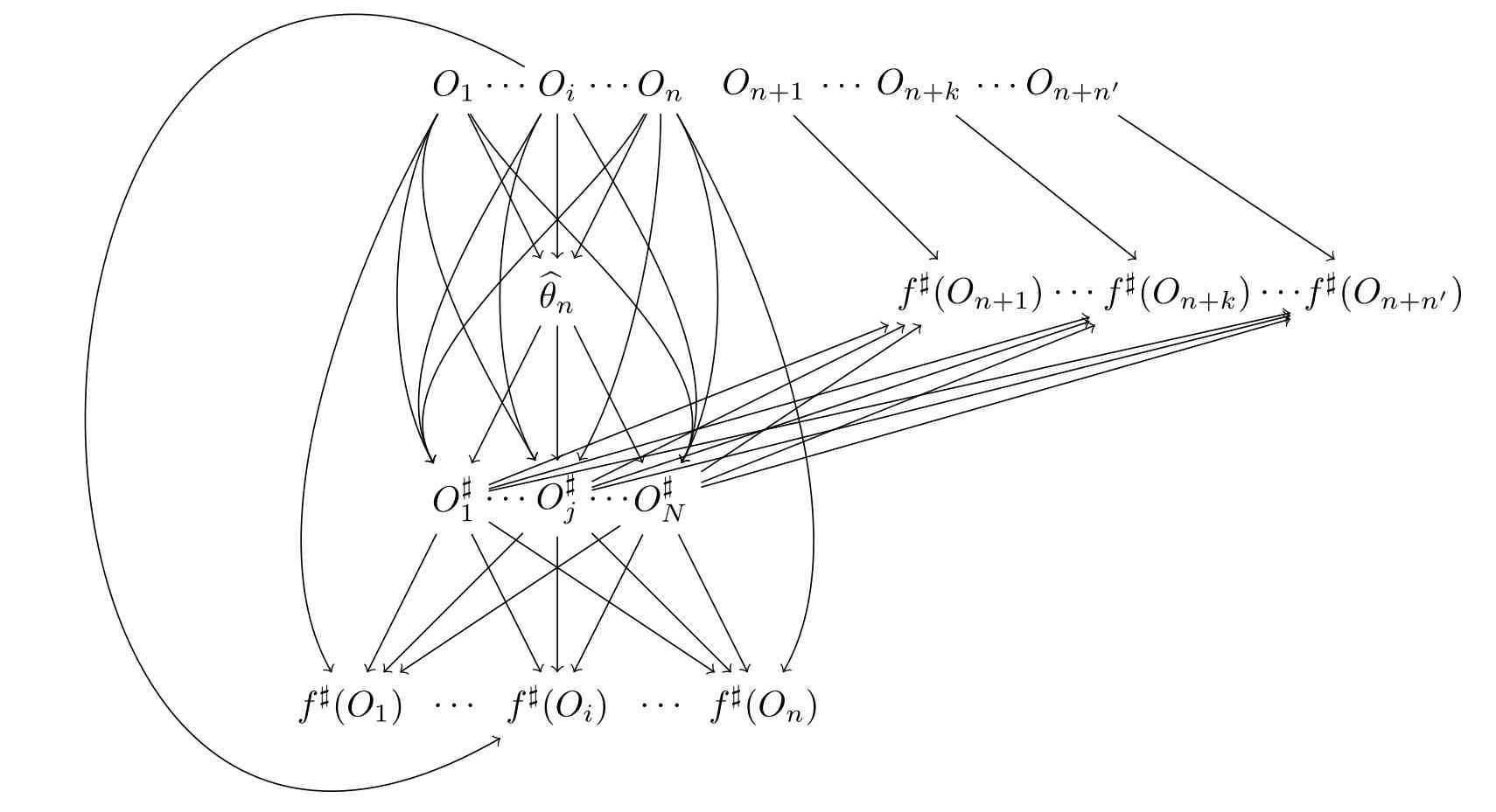{height=400}
DAG representing how the random variables produced by $\Pi$ depend on each
other.
:::
The DAG is very useful to unravel how the random variables produced by $\Pi$ depend on each other. In particular, by $d$-separation [@Lauritzen], we learn from the DAG that the distances to the nearest neighbor within $\{\Os_{1}, \ldots, \Os_{N}\}$ of $O_{1}$, $\ldots$, $O_{n+n'}$ are dependent pairwise. This dependency prevents the use of a Kolmogorov-Smirnov test to compare $\mu_{1:n}$ and $\mu_{(n+1):(n+n')}$.
Moreover, conditionally on $\Os_{1}$, $\ldots$, $\Os_{N}$,
- $O_{1}$, $\ldots$, $O_{n}$ are not independent (because, for any $1 \leq i < j \leq n$, $\Os_{1}$ is a collider on the path $O_{i} \to \Os_{1} \leftarrow O_{j}$);
- $f^{\sharp}(O_{1})$, $\ldots$, $f^{\sharp}(O_{n+n'})$ are independent (because, for any $1 \leq i < j \leq n+n'$, all paths leading from $f^{\sharp}(O_{i})$ to $f^{\sharp}(O_{j})$ are blocked);
- the distances to the nearest neighbor within $\{\Os_{1}, \ldots, \Os_{N}\}$ of $O_{n+1}$, $\ldots$, $O_{n+n'}$ are mutually independent.
Therefore, conditionally on $\Os_{1}$, $\ldots$, $\Os_{N}$ and $\mu_{1:n}$, we can use t-tests to compare the three first moments of $\mu_{(n+1):(n+n')}$ to those of $\mu_{1:n}$. By the central limit theorem and Slutsky's lemma [@vdV98, Example 2.1 and Lemma 2.8], the tests are asymptotically valid as $n'$ goes to infinity.
The next chunk of code retrieves the $p$-values of the three tests using all 1000 synthetic observations.
```{r, testing-moments-1}
(moments_test <- fig$data %>%
   dplyr::mutate(`1st_moment` = mean(fig$data %>%
                                     dplyr::filter(type == "training data") %>%
                                     dplyr::pull(d)),
                 `2nd_moment` = mean(fig$data %>%
                                     dplyr::filter(type == "training data") %>%
                                     dplyr::pull(d) %>% .^2),
                 `3rd_moment` = mean(fig$data %>%
                                     dplyr::filter(type == "training data") %>%
                                     dplyr::pull(d) %>% .^3)) %>%
   dplyr::filter(type == "testing data") %>%
   tidyr::nest() %>%
   dplyr::mutate(
              `1st_moment_test` =
                  purrr::map(data,
                             function(df)
                                 stats::t.test(df$d, mu = df$`1st_moment`[1])$p.val),
              `2nd_moment_test` =
                  purrr::map(data,
                             function(df)
                                 stats::t.test(df$d^2, mu = df$`2nd_moment`[1])$p.val),
              `3rd_moment_test` =
                  purrr::map(data,
                             function(df)
                                 stats::t.test(df$d^3, mu = df$`3rd_moment`[1])$p.val)
          ) %>%
   dplyr::select(-data) %>%
   tidyr::unnest(cols = c(`1st_moment_test`, `2nd_moment_test`, `3rd_moment_test`)))
```
The $p$-values from the first two tests are small, but not strikingly so, especially when accounting for multiple testing. This indicates only moderate evidence of a discrepancy.
It is tempting to investigate what happens when only 100 synthetic observations are used.
```{r, testing-moments-1-revisited}
(tibble::tibble(d = c(kknn::kknn(frml, train, synth %>% dplyr::slice_head(n = 100), k = 1)$D,
                      kknn::kknn(frml, test, synth %>% dplyr::slice_head(n = 100), k = 1)$D)) %>%
  dplyr::mutate(type = c(rep("training data", dplyr::n()/2),
                         rep("testing data", dplyr::n()/2))) %>%
  dplyr::mutate(`1st_moment` = mean(fig$data %>%
                                     dplyr::filter(type == "training data") %>%
                                     dplyr::pull(d)),
                 `2nd_moment` = mean(fig$data %>%
                                     dplyr::filter(type == "training data") %>%
                                     dplyr::pull(d) %>% .^2),
                 `3rd_moment` = mean(fig$data %>%
                                     dplyr::filter(type == "training data") %>%
                                     dplyr::pull(d) %>% .^3)) %>%
   dplyr::filter(type == "testing data") %>%
   tidyr::nest() %>%
   dplyr::mutate(
              `1st_moment_test` =
                  purrr::map(data,
                             function(df)
                                 stats::t.test(df$d, mu = df$`1st_moment`[1])$p.val),
              `2nd_moment_test` =
                  purrr::map(data,
                             function(df)
                                 stats::t.test(df$d^2, mu = df$`2nd_moment`[1])$p.val),
              `3rd_moment_test` =
                  purrr::map(data,
                             function(df)
                                 stats::t.test(df$d^3, mu = df$`3rd_moment`[1])$p.val)
          ) %>%
   dplyr::select(-data) %>%
   tidyr::unnest(cols = c(`1st_moment_test`, `2nd_moment_test`, `3rd_moment_test`)))
```
This time, only the $p$-value from the third tests is small, but not markedly so when accounting for multiple testing. The evidence of a discrepancy is significantly weaker when 100 synthetic observations are used compared to
1000. This highlights that distinguishing $N$ synthetic observations from genuine observations becomes increasingly difficult as $N$ decreases.
### Criterion 2
The next chunk of code implements the second criterion, in its visual form.
```{r}
#| label: fig-criterion-2
#| fig-cap: Empirical c.d.f. of each covariate based on either the synthetic or the testing data sets.
#| message: false
fig <- dplyr::bind_rows(test, synth) %>%
  dplyr::select(-Z) %>%
  dplyr::mutate(type = c(rep("testing data", dplyr::n()/2),
                         rep("synthetic data", dplyr::n()/2))) %>%
  tidyr::pivot_longer(-type, names_to = "what", values_to = "values") %>%
  dplyr::mutate(what = dplyr::case_when(
           what == "W1" ~ "W[1]",
           what == "W2" ~ "W[2]",
           what == "W3" ~ "W[3]",
           what == "V1" ~ "V[1]",
           what == "V2" ~ "V[2]",
           TRUE ~ what
  )) %>%
  dplyr::mutate(what = factor(what,
                              levels = c(paste0("W[", 1:dimW, "]"),
                                         paste0("V[", 1:dimV, "]"),
                                         "A", "Y"))) %>%
  ggplot2::ggplot() +
  ggplot2::stat_ecdf(ggplot2::aes(x = values, color = type)) +
  ggplot2::facet_wrap(~ what,
                      scales = "free_x",
                      labeller = ggplot2::label_parsed) +
  ggplot2::ylab("empirical cumulative distribution function")
print(fig)
```
Firstly, inspecting the first row of @fig-criterion-2 suggests that the marginal laws of $W_{1}, W_{2}, W_{3}$ under the synthetic law do not align very well with their counterparts under $P$, although the locations and ranges of the true marginal laws are reasonably well approximated. The restriction to $\bbR_{+}$ of the marginal law of $W_{1}$ under the synthetic law is very similar to its counterpart under $P$, but its restriction to $\bbR_{-}$ is too thin-tailed. As for the marginal laws of $W_{2}, W_{3}$ under the synthetic law, they are too thin-tailed compared to their counterparts under $P$.
Secondly, inspecting the second row of @fig-criterion-2 reveals that the marginal laws of $V_{1}, V_{2}$ under the synthetic law align perfectly ($V_{1}$) and reasonably well ($V_{2}$) with their counterparts under $P$. However, the marginal law of $A$ under the synthetic law assigns more weight to the event $[A=1]$ than its counterpart under $P$.
Lastly, inspecting the third row of @fig-criterion-2 reveals that the marginal law of $Y$ under the synthetic law does not align very well with its counterpart under $P$. While the location and range of the true marginal law are reasonably well approximated, the overall shape of the true density is not faithfully reproduced.
The next chunk of code implements the version of the second criterion based on hypotheses testing. Conditionally on the training data set, the testing procedures are valid because (i) the synthetic and testing data sets are independent, (ii) the testing data are drawn independently from $P$, (iii) the synthetic data are drawn independently from $\law(\Gen_{\thn}(Z))$.
We first address the continuous covariates ($W_1$, $W_2$, $W_3$ and $Y$) and then the binary covariates ($V_{1}$, $V_{2}$ and $A$). For the former, we use Kolmogorov-Smirnov tests. For the latter, we use exact Fisher tests.
```{r, tests-criterion-2}
#| message: false
#| warning: false
(ks_tests <- fig$data %>%
  dplyr::filter(!what %in% c(paste0("V[", 1:dimV, "]"), "A")) %>%
  tidyr::nest(data = -what) %>%
  dplyr::mutate(p.val = purrr::map(data,
                                   ~ stats::ks.test(stats::formula(values ~ type),
                                                    data = .x)$p.val)) %>%
  dplyr::select(-data) %>%
  tidyr::unnest(cols = p.val))
(fisher_test <- fig$data %>%
  dplyr::filter(what %in% c(paste0("V[", 1:dimV, "]"), "A")) %>%
  dplyr::group_by(what, type) %>%
  dplyr::summarize(`=1` = sum(values),
                   `=0` = dplyr::n()-sum(values)) %>%
  dplyr::select(-type) %>%
  tidyr::nest(data = -what) %>%
  dplyr::mutate(p.val = purrr::map(data,
                                   ~ stats::fisher.test(.x)$p.val)) %>%
  dplyr::select(-data) %>%
  tidyr::unnest(cols = p.val))
```
Most $p$-values are very small, supporting the conclusions drawn from inspecting @fig-criterion-2. Unlike the marginal laws of $V_{1}, V_{2}$, the marginal laws of $W_{1}, W_{2}, W_{3}, A, Y$ are not well approximated, as the tests detect discrepancies when both the synthetic and testing data sets contain 1000 data points.
Naturally, one might wonder whether this result still holds when comparing smaller synthetic and testing data sets. The following chunk of code reproduces the same statistical analysis as before, but now using two samples of 100 data points each.
```{r, tests-criterion-2-revisited}
#| message: false
#| warning: false
smaller_dataset <- fig$data %>%
   dplyr::group_by(type) %>%
   dplyr::slice_head(n = 100) %>%
   dplyr::ungroup()
(ks_tests <- smaller_dataset %>%
  dplyr::filter(!what %in% c(paste0("V[", 1:dimV, "]"), "A")) %>%
  tidyr::nest(data = -what) %>%
  dplyr::mutate(p.val = purrr::map(data,
                                   ~ stats::ks.test(stats::formula(values ~ type),
                                                    data = .x)$p.val)) %>%
  dplyr::select(-data) %>%
  tidyr::unnest(cols = p.val))
(fisher_test <- smaller_dataset %>%
  dplyr::filter(what %in% c(paste0("V[", 1:dimV, "]"), "A")) %>%
  dplyr::group_by(what, type) %>%
  dplyr::summarize(`=1` = sum(values),
                   `=0` = dplyr::n()-sum(values)) %>%
  dplyr::select(-type) %>%
  tidyr::nest(data = -what) %>%
  dplyr::mutate(p.val = purrr::map(data,
                                   ~ stats::fisher.test(.x)$p.val)) %>%
  dplyr::select(-data) %>%
  tidyr::unnest(cols = p.val))
```
This time, the $p$-values are large, indicating that the tests cannot detect discrepancies when the synthetic and testing data sets contain only 100 data points. Surprisingly, the same conclusion holds when comparing a synthetic data set of 100 data points with a testing data set of 1000 data points, as demonstrated in the next chunk of code.
```{r, tests-criterion-2-revisited-2}
#| message: false
#| warning: false
smaller_synth_dataset <- fig$data %>%
  dplyr::filter(type == "synthetic data") %>%
  dplyr::slice_head(n = 100) %>%
  dplyr::bind_rows(fig$data %>%
                   dplyr::filter(type == "testing data"))
(ks_tests <- smaller_synth_dataset %>%
  dplyr::filter(!what %in% c(paste0("V[", 1:dimV, "]"), "A")) %>%
  tidyr::nest(data = -what) %>%
  dplyr::mutate(p.val = purrr::map(data,
                                   ~ stats::ks.test(stats::formula(values ~ type),
                                                    data = .x)$p.val)) %>%
  dplyr::select(-data) %>%
  tidyr::unnest(cols = p.val))
(fisher_test <- smaller_synth_dataset %>%
  dplyr::filter(what %in% c(paste0("V[", 1:dimV, "]"), "A")) %>%
  dplyr::group_by(what, type) %>%
  dplyr::summarize(`=1` = sum(values),
                   `=0` = dplyr::n()-sum(values)) %>%
  dplyr::select(-type) %>%
  tidyr::nest(data = -what) %>%
  dplyr::mutate(p.val = purrr::map(data,
                                   ~ stats::fisher.test(.x)$p.val)) %>%
  dplyr::select(-data) %>%
  tidyr::unnest(cols = p.val))
```
In conclusion, while a large synthetic data set can be shown to differ in law from a large testing data set, a smaller synthetic data set does not exhibit noticeable differences in marginal laws when compared to either a small or a large testing data set.
### Criterion 3
The next chunk of code builds a super learning algorithm to estimate either the conditional probability that $A=1$ given $(W,V)$ or the conditional mean of $Y$ given $(A,W,V)$ by aggregating 5 base learners. We use the `SuperLearner` package in `R`. Specifically, the 5 base learners estimate the above conditional means by a constant (`SL.mean`), or based on generalized linear models (`SL.glm` and `SL.glm.interaction`), or by a random forest (`SL.ranger`), or based on a single-hidden-layer neural network (`SL.nnet`).
```{r, criterion-3}
#| message: false
library(SuperLearner)
algo <- function(learning_data, testing_data,
                 outcome, covariates) {
  SL.lib <- c("SL.mean", "SL.glm", "SL.glm.interaction", "SL.ranger", "SL.nnet")
  cvControl <- SuperLearner::SuperLearner.CV.control(V = 10)
  family <- switch(outcome,
                   A = stats::binomial(),
                   Y = stats::gaussian())
  sl <- SuperLearner::SuperLearner(
                        Y = dplyr::pull(learning_data, outcome),
                        X = learning_data[, covariates],
                        newX = testing_data[, covariates],
                        family = family,
                        SL.library = SL.lib,
                        method = "method.NNLS",
                        cvControl = cvControl)
  list(as.vector(sl$SL.predict))
}
```
We train the super learning algorithm three times: once on each of two distinct halves of the training data set, and once on half of the synthetic data set. This results in three estimators of the conditional probability that $A=1$ given $(W,V)$ and three estimators of the conditional mean of $Y$ given $(A,W,V)$. The next chunk of code prepares the three training data sets.
```{r, super-learning-three-times}
(tib <- dplyr::bind_rows(train, test, synth) %>%
   dplyr::select(-Z) %>%
   dplyr::mutate(type = c(rep("using training data a", dplyr::n()/6),
                          rep("using training data b", dplyr::n()/6),
                          rep("testing data a", dplyr::n()/6),
                          rep("testing data b", dplyr::n()/6),
                          rep("using synthetic data", dplyr::n()/3))) %>%
   dplyr::group_by(type) %>%
   dplyr::mutate(id = 1:dplyr::n()) %>%
   dplyr::ungroup() %>%
   dplyr::filter(id <= dplyr::n()/6) %>%
   dplyr::mutate(type = dplyr::case_when(
                                 stringr::str_detect(type, "testing") ~ "testing data",
                                 TRUE ~ type)) %>%
   dplyr::select(-id) %>%
   tidyr::nest(data = -type) %>%
   dplyr::mutate(testing = data[3]) %>%
     dplyr::filter(type != "testing data"))
```
The following chunk of code trains the super learning algorithm and evaluates the six resulting estimators on the testing data points. To compare the estimators, we use scatter plots. Specifically, denoting by $\pr_{1}, \pr_{2}, \pr_{3}$ the estimators of the conditional probability that $A=1$ given $(W,V)$ obtained by training the super learning algorithm on each of the two distinct halves of the training data set ($\pr_{1}$ and $\pr_{2}$), and on half of the synthetic data set ($\pr_{3}$), we plot in the left-hand side panel $\{(\pr_{1}(W_{n+i},V_{n+i}), \pr_{2}(W_{n+i},V_{n+i})) : 1 \leq i \leq n\}$ (in red) and $\{(\pr_{1}(W_{n+i},V_{n+i}), \pr_{3}(W_{n+i},V_{n+i})) : 1 \leq i \leq n\}$ (in blue).
Therein, the spread of the red scatter plot along the $y=x$ line in the $xy$-plane is an evidence of the inherent and irreducible randomness that one faces when one learns the conditional probability that $A=1$ given $(W,V)$. By comparison, the blue scatter plot is more widely spread around the line, revealing a measure of discrepancy between the training and synthetic data.
The right-hand side panel is obtained analogously. The red scatter plot is more concentrated around the $y=x$ line than its counterpart in the left-hand side panel. The blue scatter plot is more widely spread than the red one, which again reveals a measure of discrepancy between the training and synthetic data. In summary, we consider that the red and blue scatter plots do not strongly differ in their bulks. However, it seems that the blue scatter plots feature more outliers than their red counterparts, revealing that the estimators may be quite different in some parts of the space of covariates.
```{r}
#| label: fig-criterion-3
#| fig-cap: Comparing predicted conditional probabilities that $A=1$ given $(W,V)$ (left) or predicted conditional means of $Y$ given $(A,W,V)$ (right) when a super learning algorithm is trained twice on two distinct halves of the training data set (red points) or on the first half of the training data set, $x$-axis, and on half of the synthetic data set, $y$-axis (blue points).
#| message: false
tib %>%
  dplyr::group_by(type) %>%
  dplyr::mutate(AgivenWV = algo(data[[1]], testing[[1]],
                                "A",
                                c(paste0("W", 1:dimW),
                                  paste0("V", 1:dimV))),
                YgivenAWV = algo(data[[1]], testing[[1]],
                                 "Y",
                                 c(paste0("W", 1:dimW),
                                   paste0("V", 1:dimV),
                                   "A"))) %>%
  dplyr::ungroup() %>%
  dplyr::select(type, AgivenWV, YgivenAWV) %>%
  tidyr::unnest(cols = c(AgivenWV, YgivenAWV)) %>%
  tidyr::pivot_longer(!type, names_to = "what", values_to = "preds") %>%
  dplyr::group_by(type, what) %>%
  dplyr::mutate(id = 1:dplyr::n()) %>%
  tidyr::pivot_wider(names_from = type,
                     values_from = "preds",
                     names_prefix = "preds ") %>%
  dplyr::ungroup() %>%
  dplyr::mutate(what = dplyr::case_when(
                                what == "AgivenWV" ~ "A given (W,V)",
                                what == "YgivenAWV" ~ "Y given (A, W, V)"
                              )) %>%
  ggplot2::ggplot() +
  ggplot2::geom_point(ggplot2::aes(`preds using training data a`,
                                   `preds using synthetic data`,
                                   ),
                      color = "#00BFC4", alpha = 0.5) +
  ggplot2::geom_point(ggplot2::aes(`preds using training data a`,
                                   `preds using training data b`,
                                   ),
                      color = "#F8766D", alpha = 0.5) +
  ggplot2::geom_abline() +
  ggplot2::facet_wrap(dplyr::vars(what),
                      labeller = ggplot2::as_labeller(\(str) paste("predicting", str))) +
  ggplot2::xlab("algorithm trained on 1st half of training data set") +
    ggplot2::ylab("algorithm trained either\n
on 2nd half of training data set (red) or\n
on synthetic data set (blue)")
```
### Summary
We implement three criteria to evaluate the synthetic observations. The first criterion compared empirical distributions of distances between genuine observations, both involved and not involved in the generator's construction, and synthetic observations, detecting minor over-replication in the synthetic data set. The second criterion assessed marginal distributions of individual features, revealing discrepancies, particularly in continuous variables, which often exhibited overly thin tails. The third criterion compared predictions from an algorithm trained on synthetic versus genuine observations, showing good replication for predicting $Y$ given $(A,W,V)$ but less so for predicting $A$ given $(W,V)$. Overall, while the synthetic observations show some discrepancies from the genuine ones, these differences are not overly substantial. Moreover, detecting significant differences becomes much harder with smaller synthetic datasets (100 versus 1000 synthetic observations).
# Illustration on real data {#sec-IWPC}
In this section, we extend the analysis conducted in the previous section to real data. We use a subset of the International Warfarin Pharmacogenetics Consortium [IWPC data set](https://www.pharmgkb.org/downloads) [@IWPC]. Warfarin therapy is a commonly prescribed anticoagulant employed to treat thrombosis and thromboembolism.
## The International Warfarin Pharmacogenetics Consortium data set {#sec-pres-IWPC}
In order to limit the number of incomplete observations, we keep only the following variables:
* height, in centimeters;
* weight, in kilograms;
* indicator of whether or not VKORC1 consensus (obtained from genotype data) is "A/A";
* indicator of whether or not CYP2C9 consensus (obtained from genotype data) is "\*1/\*1";
* indicator of whether or not ethnicity is Asian;
* indicator of whether or not therapeutic dose of Warfarin is greater than or equal to 21 mg;
* international normalized ratio on reported therapeutic dose of Warfarin (INR, a measure of blood clotting function).
```{r, load-IWPC-data}
#| message: false
#| warning: false
dimW <- 2
dimV <- 3
dataset <- readr::read_csv("data/IWPC_data.csv",
                           skip = 1,
                           col_names = c("id",
                                         paste0("W", 1:dimW),
                                         paste0("V", 1:dimV),
                                         "A", "Y"))
```
The original database includes `r nrow(dataset)` patients with complete observations for these variables. We refer to the table below for a brief description of the data, and emphasize that $A$ does precede $Y$.
```{r}
#| label: tbl-descriptive-statistics-IWPC-data
#| message: false
#| warning: false
dataset %>%
    dplyr::select(V1, V2, V3, W1, W2, A, Y) %>%
    gtsummary::tbl_summary(
                   label = list(W1 = "Height (cm)",
                                W2 = "Weight (kg)",
                                V1 = "VKORC1 consensus is A/A",
                                V2 = "CYP2C9 consensus is *1/*1",
                                V3 = "Ethnicity is Asian",
                                A = "Therapeutic dose >= 21 mg per week",
                                Y = "INR"),
                   statistic = list(
                       gtsummary::all_continuous() ~ "{min}",
                       gtsummary::all_dichotomous() ~ "{n} ({p}%)"),
                   digits = list(
                       gtsummary::all_continuous() ~ rep(0, 5),
                       gtsummary::all_categorical() ~ rep(0, 2)),
                   type = list(W1 = "continuous",
                               W2 = "continuous",
                               V1 = "dichotomous",
                               V2 = "dichotomous",
                               V3 = "dichotomous",
                               A = "dichotomous",
                               Y = "continuous"),
                   value = list(V1 ~ 0, V2 ~ 0, V3 ~ 1)
               ) %>%
    gtsummary::add_stat(
                   fns = gtsummary::all_continuous() ~
                       \(data, variable, ...) stats::median(data[[variable]])
               ) %>%
    gtsummary::add_stat(
                   fns = gtsummary::all_continuous() ~
                       \(data, variable, ...) mean(data[[variable]])
               ) %>%
    gtsummary::add_stat(
                   fns = gtsummary::all_continuous() ~
                       \(data, variable, ...) max(data[[variable]])
               ) %>%
    gtsummary::add_stat(
                   fns = gtsummary::all_continuous() ~
                       \(data, variable, ...) stats::sd(data[[variable]])
               )  %>%
    gtsummary::modify_spanning_header(
                   c("variable", "label") ~
                       "**Variables**",
                   c("stat_0", "add_stat_1", "add_stat_2", "add_stat_3", "add_stat_4") ~
                       "**Descriptive statistics**") %>%
    gtsummary::modify_header(
                   variable = "", label = "", stat_0 = "**n (%) or Min**",
                   add_stat_1 = "**Median**", add_stat_2 = "**Mean**",
                   add_stat_3 = "**Max**", add_stat_4 = "**SD**") %>%
    gtsummary::modify_footnote(stat_0 = NA)
```
Let us load the data set into `Python`.
```{python, loading-real-data}
import pandas as pd

dataset = pd.read_csv("data/IWPC_data.csv")
dataset = dataset.drop(['Unnamed: 0'], axis = 1)
dataset = dataset.values
n = np.shape(dataset)[0]

dimV,  dimW = 3, 2
dimWV = dimW + dimV
nb_cat_V = np.array([len(np.unique(dataset[:, 2])),
                     len(np.unique(dataset[:, 3])),
                     len(np.unique(dataset[:, 4]))])
```
It is convenient to rescale the continuous variables.
```{python, rescaling-real-data}
#| message: false
from sklearn.preprocessing import MinMaxScaler

scalerW = MinMaxScaler(feature_range = (0, 1))
scalerW.fit(dataset[:, 0:2]);
dataset[:,0:2] = scalerW.transform(dataset[:, 0:2])

scalerY = MinMaxScaler(feature_range = (0, 1))
scalerY.fit(dataset[:, dimWV + 1].reshape(-1, 1));
dataset[:, dimWV + 1] = scalerY.transform(dataset[:, dimWV + 1].reshape(-1, 1)).reshape(1,-1)
```
We finally define the training and testing data sets.
```{python, train-test-IWPC}
n_train = int(n/2)
train = dataset[0:n_train, :]
test = dataset[n_train:n, :]
print("The three first observations in 'train':\n",
      "  V_1   V_2   V_3   W_1   W_2   A     Y\n",
      np.around(train[:3, [2, 3, 4, 0, 1, 5, 6]], decimals = 3))
```
## Training the VAE {#sec-training-VAE-IWPC}
By running the next chunk of code, we set the VAE's configuration.
```{python, vae-training-IWPC-preliminary}
latent_dim = 10
L = 8

nlayers_encoder = 2
nneurons_encoder = 8

nlayers_WV_decoder = 2
nneurons_WV_decoder = 8

nlayers_Alaw_decoder = 2
nneurons_Alaw_decoder = 8

nlayers_AYaY_decoder = 2
nneurons_AYaY_decoder = 16
```
The next chunk of code repeatedly generates and initializes a VAE then trains it.
```{python, vae-training-IWPC}
#| eval: false
  epochs = 40
  batch_size = np.round(0.2 * np.shape(train)[0]).astype(int)
  synth_size = 1000
  nb_tries = 100
  for i in range(nb_tries):
    print("try #", i, ", ")
    encoder = build_encoder(dimW = dimW,
                            dimV = dimV,
                            latent_dim = latent_dim,
                            L = L,
                            nlayers_encoder = nlayers_encoder,
                            nneurons_encoder = nneurons_encoder)
    WV_decoder = build_WV_decoder(dimW = dimW,
                                  dimV = dimV,
                                  nb_cat_V = nb_cat_V,
                                  latent_dim = latent_dim,
                                  L = L,
                                  nlayers_WV_decoder = nlayers_WV_decoder,
                                  nneurons_WV_decoder = nneurons_WV_decoder,
                                  activation_W = "sigmoid")
    Alaw_decoder = build_Alaw_decoder(dimW = dimW,
                                      dimV = dimV,
                                      L = L,
                                      nlayers_Alaw_decoder = nlayers_Alaw_decoder,
                                      nneurons_Alaw_decoder = nneurons_Alaw_decoder)
    AYaY_decoder = build_AYaY_decoder(dimW = dimW,
                                      dimV = dimV,
                                      latent_dim = latent_dim,
                                      L = L,
                                      nlayers_AYaY_decoder = nlayers_AYaY_decoder,
                                      nneurons_AYaY_decoder = nneurons_AYaY_decoder,
                                      activation_Ya = "sigmoid")
    pi = build_pi(dimW = dimW,
                  dimV = dimV,
                  L = L)
    extract_G = build_extract_G(dimW = dimW,
                                dimV = dimV,
                                L = L)
    generator = build_generator(dimW = dimW,
                                dimV = dimV,
                                encoder = encoder,
                                latent_dim = latent_dim,
                                L = L,
                                WV_decoder = WV_decoder,
                                Alaw_decoder = Alaw_decoder,
                                AYaY_decoder = AYaY_decoder,
                                pi = pi,
                                extract_G = extract_G)
    vae = VAE(generator = generator,
              latent_dim = latent_dim,
              L = L,
              optimizer = optimizer)
    vae.train(data_train = train,
              epochs = epochs,
              batch_size = batch_size)
    random_sample = np.random.choice(n_train, synth_size, replace = True)
    O_test = train[random_sample, :]
    alea = np.random.normal(loc = 0, scale = 1, size = (synth_size, L, latent_dim + dimV + 1))
    synth = vae.generator.predict([O_test, alea])[1]

    synth = synth[:, 0, :]
    synth[:, 0:2] = scalerW.inverse_transform(synth[:, 0:2])
    synth[:, dimWV + 1]\
      = scalerY.inverse_transform(synth[:, dimWV + 1].reshape(-1, 1)).reshape(1,-1)
    synth[:, 2:5] = np.round(synth[:, 2:5])
    np.savetxt("IWPC-synth_try#" + str(i) + ".csv", synth, delimiter = ",")
```
Because running the chunk is time-consuming, we stored one trained VAE that we
considered good enough. We now turn to its evaluation based on the three
criteria discussed in @sec-eval-quality and @sec-eval-quality-implemented.
## Evaluating the quality of the generator
The next chunk of code defines in `R` the counterparts `train` and `test` of
the `Python` objects `train` and `test` (keeping only the first 1000
observations), and `synth`, the collection of 1000 synthetic observations
drawn from the generator associated to the VAE that we stored in
@sec-training-VAE-IWPC. For later use (while implementing Criterion 1) we add
a dummy column named `Z`.
```{r, define-train-test-synth-data-IWPC}
#| message: false
#| warning: false
dataset <- dataset %>%
    dplyr::select(-1) %>%
    dplyr::mutate(A = as.integer(A),
                  Z = stats::rnorm(dplyr::n()))
train <- dataset %>%
    dplyr::slice_head(n = 1e3)
test <- dataset %>%
    dplyr::slice_tail(n = 1e3)
synth <- readr::read_csv("data/IWPC-synth_try#20.csv",
                         col_names = c(paste0("W", 1:dimW),
                                       paste0("V", 1:dimV),
                                       "A", "Y")) %>%
  dplyr::mutate(A = as.integer(A),
                V1 = round(V1),
                V2 = round(V2),
                V3 = round(V3),
                Z = stats::rnorm(dplyr::n()))
```
### Criterion 1
The next chunk of code implements the first criterion.
```{r}
#| label: fig-criterion-1-IWPC
#| fig-cap: Empirical c.d.f. of the distance to the nearest neighbor within the synthetic observations of the training and of the testing IWPC data points (logarithmic scale). The two c.d.f. are quite close.
#| message: false
frml <- paste0("Z ~",
               paste0(c(paste0("W", 1:dimW),
                        paste0("V", 1:dimV),
                        "A", "Y"),
                     collapse = " + ")) %>%
  stats::as.formula()
fig <- tibble::tibble(d = c(kknn::kknn(frml, train, synth, k = 1)$D,
                            kknn::kknn(frml, test, synth, k = 1)$D)) %>%
  dplyr::mutate(type = c(rep("training data", dplyr::n()/2),
                         rep("testing data", dplyr::n()/2))) %>%
  ggplot2::ggplot() +
  ggplot2::stat_ecdf(ggplot2::aes(x = d, color = type)) +
  ggplot2::scale_x_log10() +
  ggplot2::xlab("distance to nearest neighbor") +
  ggplot2::ylab("empirical cumulative distribution function")
print(fig)
```
The two empirical c.d.f. shown in @fig-criterion-1-IWPC are not as similar as
those in @fig-criterion-1. The next chunk of code implements the t-tests
comparing the three first moments of $\mu_{(n+1):(n+n')}$ to those of
$\mu_{1:n}$.
```{r, testing-moments-1-IPW}
(moments_test <- fig$data %>%
   dplyr::mutate(`1st_moment` = mean(fig$data %>%
                                     dplyr::filter(type == "training data") %>%
                                     dplyr::pull(d)),
                 `2nd_moment` = mean(fig$data %>%
                                     dplyr::filter(type == "training data") %>%
                                     dplyr::pull(d) %>% .^2),
                 `3rd_moment` = mean(fig$data %>%
                                     dplyr::filter(type == "training data") %>%
                                     dplyr::pull(d) %>% .^3)) %>%
   dplyr::filter(type == "testing data") %>%
   tidyr::nest() %>%
   dplyr::mutate(
              `1st_moment_test` =
                  purrr::map(data,
                             function(df)
                                 stats::t.test(df$d, mu = df$`1st_moment`[1])$p.val),
              `2nd_moment_test` =
                  purrr::map(data,
                             function(df)
                                 stats::t.test(df$d^2, mu = df$`2nd_moment`[1])$p.val),
              `3rd_moment_test` =
                  purrr::map(data,
                             function(df)
                                 stats::t.test(df$d^3, mu = df$`3rd_moment`[1])$p.val)
          ) %>%
   dplyr::select(-data) %>%
   tidyr::unnest(cols = c(`1st_moment_test`, `2nd_moment_test`, `3rd_moment_test`)))
```
The numerical evidence of discrepancy is compelling. But is it still as
compelling when only 100 synthetic observations are used? The next chunk of
code addresses this question.
```{r, testing-moments-1-revisited-IWPC}
(tibble::tibble(d = c(kknn::kknn(frml, train, synth %>% dplyr::slice_head(n = 100), k = 1)$D,
                      kknn::kknn(frml, test, synth %>% dplyr::slice_head(n = 100), k = 1)$D)) %>%
  dplyr::mutate(type = c(rep("training data", dplyr::n()/2),
                         rep("testing data", dplyr::n()/2))) %>%
  dplyr::mutate(`1st_moment` = mean(fig$data %>%
                                     dplyr::filter(type == "training data") %>%
                                     dplyr::pull(d)),
                 `2nd_moment` = mean(fig$data %>%
                                     dplyr::filter(type == "training data") %>%
                                     dplyr::pull(d) %>% .^2),
                 `3rd_moment` = mean(fig$data %>%
                                     dplyr::filter(type == "training data") %>%
                                     dplyr::pull(d) %>% .^3)) %>%
   dplyr::filter(type == "testing data") %>%
   tidyr::nest() %>%
   dplyr::mutate(
              `1st_moment_test` =
                  purrr::map(data,
                             function(df)
                                 stats::t.test(df$d, mu = df$`1st_moment`[1])$p.val),
              `2nd_moment_test` =
                  purrr::map(data,
                             function(df)
                                 stats::t.test(df$d^2, mu = df$`2nd_moment`[1])$p.val),
              `3rd_moment_test` =
                  purrr::map(data,
                             function(df)
                                 stats::t.test(df$d^3, mu = df$`3rd_moment`[1])$p.val)
          ) %>%
   dplyr::select(-data) %>%
   tidyr::unnest(cols = c(`1st_moment_test`, `2nd_moment_test`, `3rd_moment_test`)))
```
The strength of evidence has dropped considerably, reflected by the larger
$p$-values compared to earlier results. As in @sec-eval-quality-implemented,
distinguishing $N$ synthetic observations from genuine observations becomes
more challenging when $N=100$ compared to $N=1000$.
### Criterion 2
The next chunk of code implements the second criterion, in its visual form.
```{r}
#| label: fig-criterion-2-IWPC
#| fig-cap: Empirical c.d.f. of each covariate based on either the synthetic observations or the testing IPWC data set.
#| message: false
fig <- dplyr::bind_rows(test, synth) %>%
  dplyr::select(-Z) %>%
  dplyr::mutate(type = c(rep("testing data", dplyr::n()/2),
                         rep("synthetic data", dplyr::n()/2))) %>%
  tidyr::pivot_longer(-type, names_to = "what", values_to = "values") %>%
  dplyr::mutate(what = dplyr::case_when(
           what == "W1" ~ "W[1]",
           what == "W2" ~ "W[2]",
           what == "V1" ~ "V[1]",
           what == "V2" ~ "V[2]",
           what == "V3" ~ "V[3]",
           TRUE ~ what
  )) %>%
  dplyr::mutate(what = factor(what,
                              levels = c(paste0("W[", 1:dimW, "]"),
                                         paste0("V[", 1:dimV, "]"),
                                         "A", "Y"))) %>%
  ggplot2::ggplot() +
  ggplot2::stat_ecdf(ggplot2::aes(x = values, color = type)) +
  ggplot2::facet_wrap(~ what,
                      scales = "free_x",
                      labeller = ggplot2::label_parsed) +
  ggplot2::ylab("empirical cumulative distribution function")
print(fig)
```
@fig-criterion-2-IWPC suggests that except for $V_2$, $A$ and, to a lesser
extent, $V_1$, the marginal laws under the synthetic law do not align well
with their counterparts under $P$. This is confirmed by the following
(Kolmogorov-Smirnov or exact Fisher) hypotheses tests:
```{r, tests-criterion-2-IWPC}
#| message: false
#| warning: false
(ks_tests <- fig$data %>%
  dplyr::filter(!what %in% c(paste0("V[", 1:dimV, "]"), "A")) %>%
  tidyr::nest(data = -what) %>%
  dplyr::mutate(p.val = purrr::map(data,
                                   ~ stats::ks.test(stats::formula(values ~ type),
                                                    data = .x)$p.val)) %>%
  dplyr::select(-data) %>%
  tidyr::unnest(cols = p.val))
(fisher_test <- fig$data %>%
  dplyr::filter(what %in% c(paste0("V[", 1:dimV, "]"), "A")) %>%
  dplyr::group_by(what, type) %>%
  dplyr::summarize(`=1` = sum(values),
                   `=0` = dplyr::n()-sum(values)) %>%
  dplyr::select(-type) %>%
  tidyr::nest(data = -what) %>%
  dplyr::mutate(p.val = purrr::map(data,
                                   ~ stats::fisher.test(.x)$p.val)) %>%
  dplyr::select(-data) %>%
  tidyr::unnest(cols = p.val))
```
One might again question whether this result persists when comparing smaller
synthetic and testing datasets. The next chunk of code replicates the previous
statistical analysis, this time using two samples of 100 data points each.
```{r, tests-criterion-2-revisited-IWPC}
#| message: false
#| warning: false
smaller_dataset <- fig$data %>%
   dplyr::group_by(type) %>%
   dplyr::slice_head(n = 100) %>%
   dplyr::ungroup()
(ks_tests <- smaller_dataset %>%
  dplyr::filter(!what %in% c(paste0("V[", 1:dimV, "]"), "A")) %>%
  tidyr::nest(data = -what) %>%
  dplyr::mutate(p.val = purrr::map(data,
                                   ~ stats::ks.test(stats::formula(values ~ type),
                                                    data = .x)$p.val)) %>%
  dplyr::select(-data) %>%
  tidyr::unnest(cols = p.val))
(fisher_test <- smaller_dataset %>%
  dplyr::filter(what %in% c(paste0("V[", 1:dimV, "]"), "A")) %>%
  dplyr::group_by(what, type) %>%
  dplyr::summarize(`=1` = sum(values),
                   `=0` = dplyr::n()-sum(values)) %>%
  dplyr::select(-type) %>%
  tidyr::nest(data = -what) %>%
  dplyr::mutate(p.val = purrr::map(data,
                                   ~ stats::fisher.test(.x)$p.val)) %>%
  dplyr::select(-data) %>%
  tidyr::unnest(cols = p.val))
```
This time, except for $W_{2}$, the $p$-values are large, indicating that the
tests cannot detect discrepancies when the synthetic and testing data sets
each contain only 100 data points. As observed in
@sec-eval-quality-implemented, a similar conclusion holds when comparing a
synthetic dataset of 100 data points with a testing dataset of 1000 data
points, with $Y$ now also associated with a small $p$-value. This is
demonstrated by the next chunk of code.
```{r, tests-criterion-2-revisited-2-IWPC}
#| message: false
#| warning: false
smaller_synth_dataset <- fig$data %>%
  dplyr::filter(type == "synthetic data") %>%
  dplyr::slice_head(n = 100) %>%
  dplyr::bind_rows(fig$data %>%
                   dplyr::filter(type == "testing data"))
(ks_tests <- smaller_synth_dataset %>%
  dplyr::filter(!what %in% c(paste0("V[", 1:dimV, "]"), "A")) %>%
  tidyr::nest(data = -what) %>%
  dplyr::mutate(p.val = purrr::map(data,
                                   ~ stats::ks.test(stats::formula(values ~ type),
                                                    data = .x)$p.val)) %>%
  dplyr::select(-data) %>%
  tidyr::unnest(cols = p.val))
(fisher_test <- smaller_synth_dataset %>%
  dplyr::filter(what %in% c(paste0("V[", 1:dimV, "]"), "A")) %>%
  dplyr::group_by(what, type) %>%
  dplyr::summarize(`=1` = sum(values),
                   `=0` = dplyr::n()-sum(values)) %>%
  dplyr::select(-type) %>%
  tidyr::nest(data = -what) %>%
  dplyr::mutate(p.val = purrr::map(data,
                                   ~ stats::fisher.test(.x)$p.val)) %>%
  dplyr::select(-data) %>%
  tidyr::unnest(cols = p.val))
```
In conclusion, although a large synthetic dataset can be shown to differ in
distribution from a large testing dataset, a smaller synthetic dataset does
not display clear differences in marginal distributions (apart from $W_{3}$
and potentially $Y$) when compared to a small testing dataset.
### Criterion 3
The next chunk of code builds a super learning algorithm to estimate either
the conditional probability that $A=1$ given $(W,V)$ or the conditional mean
of $Y$ given $(A,W,V)$ by aggregating the same 5 base learners as in
@sec-eval-quality-implemented.
```{r, criterion-3-IWPC}
#| message: false
library(SuperLearner)
algo <- function(learning_data, testing_data,
                 outcome, covariates) {
  SL.lib <- c("SL.mean", "SL.glm", "SL.glm.interaction", "SL.ranger", "SL.nnet")
  cvControl <- SuperLearner::SuperLearner.CV.control(V = 10)
  family <- switch(outcome,
                   A = stats::binomial(),
                   Y = stats::gaussian())
  sl <- SuperLearner::SuperLearner(
                        Y = dplyr::pull(learning_data, outcome),
                        X = learning_data[, covariates],
                        newX = testing_data[, covariates],
                        family = family,
                        SL.library = SL.lib,
                        method = "method.NNLS",
                        cvControl = cvControl)
  list(as.vector(sl$SL.predict))
}
```
We train the super learning algorithm three times: once on each of two
distinct halves of the training data set, and once on half of the synthetic
data set. This results in three estimators of the conditional probability
that $A=1$ given $(W,V)$ and three estimators of the conditional mean of $Y$
given $(A,W,V)$. The next chunk of code prepares the three training data sets.
```{r, super-learning-three-times-IWPC}
(tib <- dplyr::bind_rows(train, test, synth) %>%
   dplyr::select(-Z) %>%
   dplyr::mutate(type = c(rep("using training data a", dplyr::n()/6),
                          rep("using training data b", dplyr::n()/6),
                          rep("testing data a", dplyr::n()/6),
                          rep("testing data b", dplyr::n()/6),
                          rep("using synthetic data", dplyr::n()/3))) %>%
   dplyr::group_by(type) %>%
   dplyr::mutate(id = 1:dplyr::n()) %>%
   dplyr::ungroup() %>%
   dplyr::filter(id <= dplyr::n()/6) %>%
   dplyr::mutate(type = dplyr::case_when(
                                 stringr::str_detect(type, "testing") ~ "testing data",
                                 TRUE ~ type)) %>%
   dplyr::select(-id) %>%
   tidyr::nest(data = -type) %>%
   dplyr::mutate(testing = data[3]) %>%
   dplyr::filter(type != "testing data"))
```
The following chunk of code trains the super learning algorithm and evaluates
the six resulting estimators on the testing data points. To compare the
estimators, we use scatter plots in the same manner as in
@sec-eval-quality-implemented.
```{r}
#| label: fig-criterion-3-IWPC
#| fig-cap: Comparing predicted conditional probabilities that $A=1$ given $(W,V)$ (left) or predicted conditional means of $Y$ given $(A,W,V)$ (right) when a super learning algorithm is trained twice on two distinct halves of the training IWPC data set (red points) or on the first half of the training IWPC data set, $x$-axis, and on half of the synthetic data set, $y$-axis (blue points).
#| message: false
#| warning: false
tib %>%
  dplyr::group_by(type) %>%
  dplyr::mutate(AgivenWV = algo(data[[1]], testing[[1]],
                                "A",
                                c(paste0("W", 1:dimW),
                                  paste0("V", 1:dimV))),
                YgivenAWV = algo(data[[1]], testing[[1]],
                                 "Y",
                                 c(paste0("W", 1:dimW),
                                   paste0("V", 1:dimV),
                                   "A"))) %>%
  dplyr::ungroup() %>%
  dplyr::select(type, AgivenWV, YgivenAWV) %>%
  tidyr::unnest(cols = c(AgivenWV, YgivenAWV)) %>%
  tidyr::pivot_longer(!type, names_to = "what", values_to = "preds") %>%
  dplyr::group_by(type, what) %>%
  dplyr::mutate(id = 1:dplyr::n()) %>%
  tidyr::pivot_wider(names_from = type,
                     values_from = "preds",
                     names_prefix = "preds ") %>%
  dplyr::ungroup() %>%
  dplyr::mutate(what = dplyr::case_when(
                                what == "AgivenWV" ~ "A given (W,V)",
                                what == "YgivenAWV" ~ "Y given (A, W, V)"
                              )) %>%
  ggplot2::ggplot() +
  ggplot2::geom_point(ggplot2::aes(`preds using training data a`,
                                   `preds using synthetic data`,
                                   ),
                      color = "#00BFC4", alpha = 0.5) +
  ggplot2::geom_smooth(ggplot2::aes(`preds using training data a`,
                                    `preds using synthetic data`,
                                   ),
                      color = "blue", method = "lm", se = FALSE) +
  ggplot2::geom_point(ggplot2::aes(`preds using training data a`,
                                   `preds using training data b`,
                                   ),
                      color = "#F8766D", alpha = 0.5) +
  ggplot2::geom_smooth(ggplot2::aes(`preds using training data a`,
                                    `preds using training data b`,
                                   ),
                      color = "red", method = "lm", se = FALSE) +
  ggplot2::geom_abline() +
    ggplot2::facet_wrap(
                 dplyr::vars(what),
                 scales = "free",
                 labeller = ggplot2::as_labeller(\(str) paste("predicting", str))
             ) +
  ggplot2::xlab("algorithm trained on 1st half of training data set") +
    ggplot2::ylab("algorithm trained either\n
on 2nd half of training data set (red) or\n
on synthetic data set (blue)")
```
Therein, the spread and asymmetry of the red scatter plot along the $y=x$ line
in the $xy$-plane are evidences of how difficult it is to estimate the
conditional probability that $A=1$ given $(W,V)$. To ease comparisons, we
also superimpose the regression lines obtained by fitting two separate linear
models on the blue and red data points. By comparison, the blue scatter plot
is less widely spread than the red one, around the blue line which deviates
more from the $y=x$ line than the red one.
The right-hand side panel is obtained analogously. The red scatter plot is
more concentrated around the $y=x$ line than its counterpart in the left-hand
side panel. This indicates that it is less difficult to estimate the
conditional mean of $Y$ given $(A,W,V)$ than the probability that $A=1$ given
$(W,V)$. The blue scatter plot is more widely spread than the red one, which
again reveals a measure of discrepancy between the training and synthetic
data. This is counterbalanced by the fact that the blue regression line
almost coincides with the $y=x$ line, whereas the red one deviates from it.
## Summary
We implemented the same three criteria as in
@sec-eval-quality-implemented. Overall, the synthetic observations showed more
substantial discrepancies from the IWPC (genuine) ones compared to the
analysis on simulated data. Furthermore, detecting significant differences
remained challenging with smaller synthetic datasets (100 versus 1000
synthetic observations), but the gaps were more evident in the real-data
context.
# Conclusion {#sec-conclusion}
This final section contextualizes our study by reviewing related works,
discussing the challenges and limitations encountered, and offering a closing
reflection on the broader implications of our approach and findings.
## Related works
Before the advent of neural networks, synthetic tabular data were typically
generated by modeling the joint law of genuine tabular data and sampling from
it. The parametric models involved canonical distributions and were often
restricted to low-dimensional settings, due to computational limitations and
the challenges of effectively encoding large, parameterized classes of
functions.
With the emergence of neural networks, numerous studies have focused on
generating synthetic data across diverse fields, including image generation
[@yi_2019], video synthesis [@vondrick_2016], natural language processing
[@lee_2018], and healthcare [@che_2017], [@choi_2017], [@baowaly_2018],
[@lee_2018], [@yi_2019]. Most of these studies employed Generative Adversarial
Networks (GANs, @goodfellow_generative_2014), as seen in works such as
[@creswell_2017], [@gui_2020], [@aggarwal_2021], [@figueira_2022]. However,
VAEs and their extensions, as well as techniques like normalizing flows
[@rezende_2015] and nonequilibrium thermodynamics [@dickstein_2015], were also
utilized.
For instance, @xu_2019 proposed the Conditional Tabular GAN (CTGAN) to address
challenges specific to tabular data, such as the mix of discrete and
continuous variables, multiple modes in continuous variables, and imbalanced
discrete variables. Their approach included mode-specific normalization,
architectural modifications, a conditional generator, and training-by-sampling
to improve performance. Additionally, they introduced the Tabular Variational
Auto-Encoder (TVAE) for mixed-type tabular data generation.
Inspired by a randomized controlled trial (RCT) in the treatment of Human
Immunodeficiency Virus (HIV), @petrakos_2025 recently conducted an empirical
comparison of several strategies and two data generation techniques aimed at
generating synthetic tabular RCT data while preserving the underlying
multivariate data distribution. One of these techniques was based on the
aforementioned CTGAN, and the other on a more traditional statistical method.
Their findings indicate that the most effective approach for generating
synthetic RCT data involves a sequential generation process. This process
begins with an R-vine copula model to generate baseline variables, followed by
a simple random treatment allocation to simulate the RCT environment, and
concludes with regression models for post-treatment variables, such as the
trial outcome.
In a causal framework, @kocaoglu_2017 proposed an adversarial training
procedure to learn a causal implicit generative model for a given causal
graph. They demonstrated that when the generator's structure aligns with the
causal graph, GANs can effectively train causal implicit generative
models. Their approach involved a two-stage procedure: first, they trained a
causal implicit generative model over binary labels using a Wasserstein GAN
(WGAN, @arjovsky_2017, @gulrajani_2017) consistent with the causal graph as
the generator. Next, they introduced a novel conditional GAN architecture,
called CausalGAN, which incorporates an anti-labeler network alongside a
labeler network in its loss function. They showed that this architecture
enables sampling from the correct conditional and interventional
distributions.
Works more similar to ours include the following. @athey_2024 proposed using
GANs to generate synthetic data that mimic genuine data, aimed at assessing
the performance of statistical methods. To illustrate their approach, they
employed WGANs to generate the covariates $(V,W)$ conditional on the treatment
$A$, followed by the outcome variable $Y$ conditional on $A$. The resulting
synthetic data were used to estimate average treatment effects.
@neal_2020 presented RealCause, an alternative approach to simulate realistic
data using neural networks. Unlike our approach, they first sampled $(V,W)$
directly from the genuine data and then generated samples for $A$
(conditionally on $(W,V)$) and $Y$ (conditionally on $(A,W,V)$).
@parikh_2022 introduced Credence, a deep generative model-based framework for
evaluating causal inference methods. A distinctive feature of their approach
is its ability to specify ground truth for both the form and magnitude of
causal effects and confounding bias as functions of covariates. Like us, they
used a VAE but modeled the joint law of $(V,W,A,Y)$ by decomposing it into the
two conditional laws of $Y$ given $(A,W,V)$ and of $(V,W)$ given $A$, along
with the marginal law of $A$. However, their decomposition of the likelihood
differs from ours.
Naturally, researchers have also focused on evaluating the quality of
synthetic data. For instance, @ahmedalaa_2022 proposed three metrics
($\alpha$-precision, $\beta$-recall, authenticity) to assess the fidelity,
diversity, and generalization performance of data generators. In their work,
each sample is individually classified as either high-quality or low-quality.
To conclude, @lu_2024 provided a comprehensive systematic review of studies
utilizing machine learning models to generate synthetic data, offering a
valuable synthesis of the field's progress and challenges.
## Challenges and limitations
The question of what volume of data is required is important. It is widely
accepted that "the more data, the better." However, this simple adage
overlooks the need to explicitly link the required data volume to both (i) the
size and complexity of the input data, and (ii) the complexity of the neural
network being fitted. In this study, we chose to (i) simulate five times as
many genuine observations as the number of observations in the IWPC real data
example, and (ii) build neural networks of comparable complexity in both
illustrations (see @sec-sim-data, @sec-IWPC). When testing our approach to
building a simulator on simulated data, we found that increasing the sample
size of the genuine observations by two- to threefold, and moderately
augmenting the complexity of the neural network (e.g., by adding one or two
more layers to the encoder and each component of the decoder and/or by
doubling the number of neurons in each layer), did not lead to significant
changes in the quality of the results.
The choice of architecture is, in a sense, a meta-hyperparameter. In
addition, several other hyperparameters must be selected by the data
scientist, including the number of layers, the number of neurons per layer,
$\beta$, and the parameters used in Algorithm 1. It is certain that the
architecture can be improved on a case-by-case basis. The data scientist's
task could benefit from input from domain experts. As for the other
hyperparameters, we do not claim that our choices are optimal. However,
selecting appropriate optimality criteria and optimizing the choices based on
them are challenging tasks.
The results of our study, while informative, are somewhat disappointing. As
reported in the first paragraph of this section, increasing the quantity of
genuine data substantially did not improve the simulator's performance in this
context. This is in stark contrast to fields like image generation, where the
abundance of inherent regularities in visual patterns enables models to learn
effectively from larger datasets. In our case, the limited improvement may
stem from a lack of rich regularities in the genuine data, which constrains
the simulator's ability to capture meaningful structures.
Another challenge lies in the question of sharing the simulator, which has
implications for privacy-preserving analytics. While making the simulator
widely available would be appealing, it raises concerns about the genuine data
required to run the code. This dependency could potentially compromise the
privacy or utility of the original dataset, creating additional barriers to
adoption.
It is also worth noting that we deliberately neutralized in this article the
VAE's repeated training from random initializations due to the high
computational time required. This is telling to the extent that the
computational cost underscores a practical limitation of the approach: the
trade-off between feasibility and the potential benefits of repeated and
extended training cycles, which might otherwise improve the simulator's
performance.
Looking ahead, addressing some of these limitations requires practical and
theoretical advances. For instance, future efforts could focus on effectively
handling missing data (NA values) within the simulation
framework. Additionally, establishing general design principles for simulator
architectures could improve their robustness and adaptability across a variety
of datasets and applications. Moreover, it would be interesting to
investigate how the notion of energy scores of @gneiting_2007 may be used to
develop new criteria to evaluate a generator's performance. The potential
relevance of our study in the context of simulation-based inference in
Bayesian computation presents another promising avenue for future work.
::: {.callout-note appearance="simple"}
## Take-home message
We highlighted key considerations in designing and testing simulators. First,
we emphasized that simply increasing the volume of data does not guarantee
improved simulator performance, especially when the data lacks rich
regularities. We also discussed the complexities of composing the right
architecture for the neural network and selecting appropriate hyperparameters
to train it. Although it is tempting to rely on larger datasets and more
complex models, increasing the data size or network complexity did not
significantly improve the results. Additionally, we touched upon the
challenges of sharing simulators, particularly in the context of
privacy-preserving analytics, where data dependencies may raise privacy
concerns. We also noted the computational burden of training, which limits the
feasibility of repeated training cycles. Finally, while our approach
addresses some of these challenges, future efforts should focus on handling
missing data, developing universal design principles for simulator
architectures, elaborating new criteria of a generator's performance, and
exploring the potential relevance of our study in the context of
simulation-based inference in Bayesian computation.
:::
## Closing reflection
As we reflect on the limitations and implications of simulators, it is worth
revisiting the paragraph in @sec-draw-me-a-model where we state that
parametric simulators "cannot convincingly replicate the multifaceted
interactions and variability inherent in 'nature'". The lexical field
surrounding "nature" itself warrants reflection.
Historically, the notion of "nature" has evolved significantly. In ancient
Greece, philosophers used the term "physis", nowadays often translated as
"nature", to explore the inherent essence or intrinsic qualities of things.
"Natura", the Roman adaptation, extended these ideas, while medieval thought
integrated nature into theological frameworks, portraying it as divine
creation.
Often regarded as a figure of the late Renaissance and an early architect of
the Scientific Revolution, Bacon emphasized in 1620 the idea of conquering
nature, viewing it as an object to be studied, understood, and controlled --
"for nature is only to be commanded by obeying her" [@Bacon]. During the
Enlightenment, the concept of "nature" further shifted, increasingly
separating it from humanity and framing it as an object of scientific study
and exploitation. These developments have frequently served as a conceptual
tool to justify humanity's dominion and looting of the non-human world.
In this context, referring to "nature" as something simulations seek to
imitate is a testament to the evolving notion of "nature," now encompassing
phenomena like human health. This shift should be questioned, especially if it
follows the Enlightenment logic of treating "nature" as an object to be
understood, controlled, and exploited. Applying such a framework to humans
risks reducing individuals to abstract data points or exploitable systems,
ignoring their intrinsic complexity and moral agency.
Recognizing these risks invites us to critically examine not only the
limitations of simulators but also their ethical and philosophical
implications. Among these are the challenges posed by a lack of fair
representability in the data used to train algorithms, which can perpetuate
existing inequities or create new ones. Fairness becomes a central issue,
particularly when simulations influence decisions that affect diverse
populations, as the underlying models may not account for all relevant
perspectives or experiences. Furthermore, the use of advanced simulations can
contribute to elitism, as access to the expertise and computational resources
needed to develop and deploy such systems is far from being universal, with
numerous countries facing more urgent challenges. Finally, the environmental
and financial cost of training complex algorithms, particularly those based on
generative AI, raises questions about sustainability and the trade-offs
between progress and resource consumption.
Fiction has always provided a space to explore hypothetical scenarios that
might be impractical, impossible, or even unethical in reality. Utopian and
dystopian literature, for example, simulates alternative societies to test
ideas about governance, morality, and human behavior. Similarly, speculative
fiction pushes boundaries by imagining futures shaped by scientific and
technological advancements. In doing so, fiction serves as a conceptual
laboratory, allowing its creators and audiences to investigate possibilities
and their consequences. This creative exploration, which has long shaped human
understanding, should continue to inform and inspire the design and purpose of
computer simulations.
# Acknowledgements
A number of open-source libraries made this work possible. In `Python`, we
relied on the packages `numpy` [@numpy], `pandas` [@pandas], `random`
[@van1995python], `sklearn` [@sklearn] and `tensorflow`
[@tensorflow2015-whitepaper]. In `R`, we used the packages `gtsummary`
[@gtsummary], `kknn` [@kknn], `SuperLearner` [@SuperLearner] and `tidyverse`
[@tidyverse]. We are grateful to the developers and maintainers of these
packages for their contributions to the research community.
The authors warmly thank Isabelle Drouet (Sorbonne Université) and Alexander
Reisach (Université Paris Cité) for their valuable feedback and insightful
comments on this project.
<!-- ```{r session-info} sessionInfo() ``` -->